Benchmark Problem #2: Three-dimensional submarine solid block

This benchmark problem is based on the 3D laboratory experiments of Enet and Grilli (2007) . Figure 2.1 shows the definitions of the key parameters and variables.

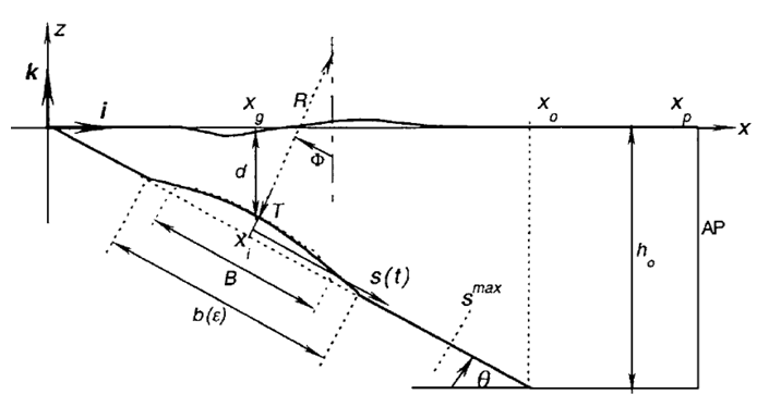
Fig. 2.1: Sketch of main parameters and variables for wave generation by 2D slide. [from Grilli and Watts, 2005]

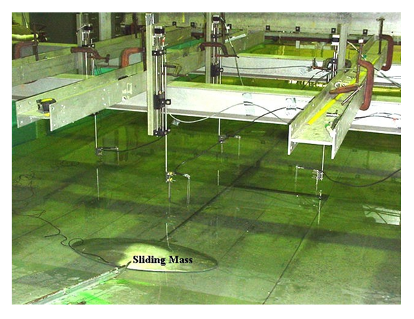
Fig. 2.2: Wave generation by underwater 3D slide. Experimental set-up for Enet and Grilli's (2007) experiments.

Figure 2.2 shows a picture of the experiments, which were performed in the University of Rhode Island (URI) fresh water wave tank (width 3.6 m, length 30 m and depth 1.8 m). The model slide slid down a plane slope built in the tank with an angle θ = 15 deg. The submarine slide model was built as a streamlined Gaussian-shaped aluminum body (Figure 2.3) with elliptical footprint, of down-slope length b = 0.395, cross-slope width w = 0.680 m, and maximum thickness T = 0.082 m. Slide shape was defined as (Figure 2.3)

Fig. 2.3: Wave generation by underwater 3D slide. Vertical cross-sections in landslide model geometry defined by Eq. (1) (dimensions are in meters).

where (ξ, χ) are the local down-slope and span-wise coordinates. With this geometry and parameters, the slide volume was found by integration as,

This volume was measured after fabricating the slide, to V_b = 7.72 x 10^-3 m³, which using the above equations and slide geometric data yields, ε = 0.717 (for which the coefficient of V_b in Eq. 2 is 0.3508).

The slide was released at time t = 0 from a series of 7 initial submergence depths d (Figure 2.1; Table 2.1). During its motion, the slide was guided by a rail located on the slope/tank axis, using low friction wheels, and slid a short distance (4 mm) above the plane slope. For each submergence depth d, the slide initial abscissa x_i and the abscissa of the slide point of maximum thickness x_g are defined and related as,

with T' = T + 0.004 (m). The slide had a central cavity housing the micro-accelerometer, which partly filled with water. Taking this into consideration, slide mass was measured as M_b = ρ_bV_b = 16.00 kg, and its bulk density (based on measured volume) was ρ_b = 2.073 kg/m³.

Measured data included: (i) slide kinematics, obtained from a composite of the slide acceleration measured using a micro-accelerometer embedded within the slide, as well as the time of passage of the slide through three electromechanical gates (see Enet and Grilli, 2007, for details); (ii) surface elevation at up to four capacitance wave gages g1 to g4 (Figure 2.4); and (iii) wave runup R_u on the slope (i.e., maximum vertical elevation on the slope), at the tank axis (y = 0). Wave gage g1 was moved in between each experiment to always be located at (x = x₀, y = 0); the coordinates of the other gages' locations in the horizontal plane (x, y) are given in Table 2.2.

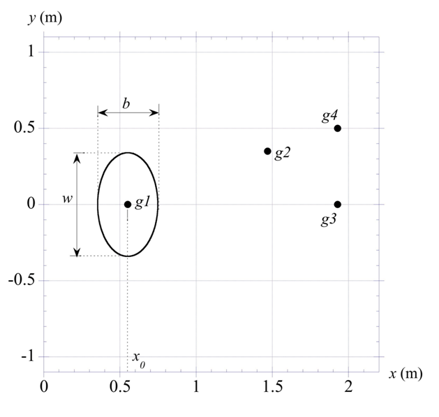
Fig. 2.4: Wave generation by underwater 3D slide. Landslide and gage locations (Table 2.2). Figure is drawn for case.

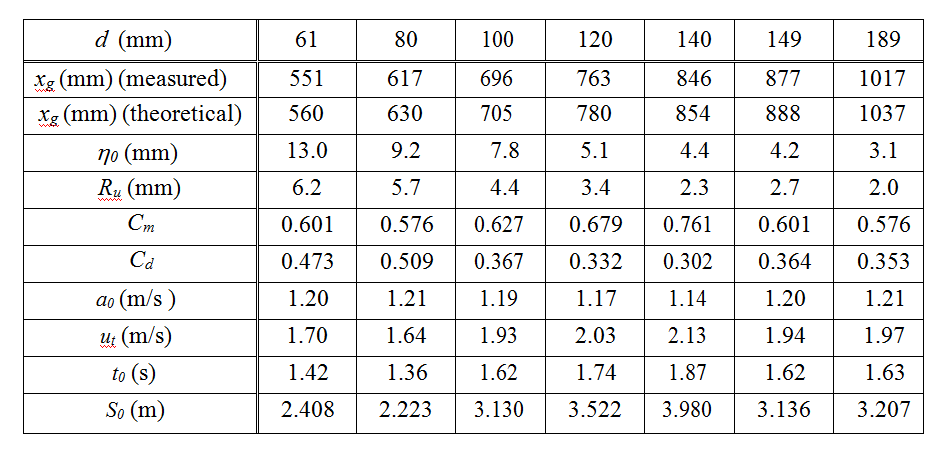
Table. 2.1: Wave generation by underwater 3D slide. Measured and curve-fitted slide and wave parameters for various slide initial submergence depths (Figure 2.1).

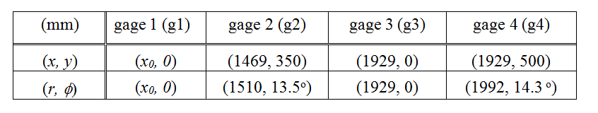
Table. 2.2: Wave generation by underwater 3D slide. Wave Gauges Locations (Figure 2.4). The second line is polar coordinates.

The measured slide kinematics was found to well match the theoretical law of motion Eqs. (1-2 for Benchmark #1) derived for slides, with the terminal velocity and initial acceleration defined as,

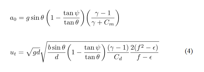
where g is gravitational acceleration, γ=ρ_b/ρ_w is the slide density, C_m is the slide added mass coefficient, C_d the slide drag coefficient, and C_n = tan ψ, the slide basal Coulomb friction. Based on Eq. (4), for ε = 0.717, we find C = 0.8616 and f = 0.8952. In each experiment, the hydrodynamic coefficients C_m and C_d were calculated as least-square fits, by applying Eqs. (1-2 for Benchmark #1, 4) to the measured slide kinematics (Figure 2.5), expressed as a composite of center of mass acceleration and time of passage at the known position of the 3 electromechanical gates (see, Enet and Grilli, 2007, for details). Results are given in Table 2.1.

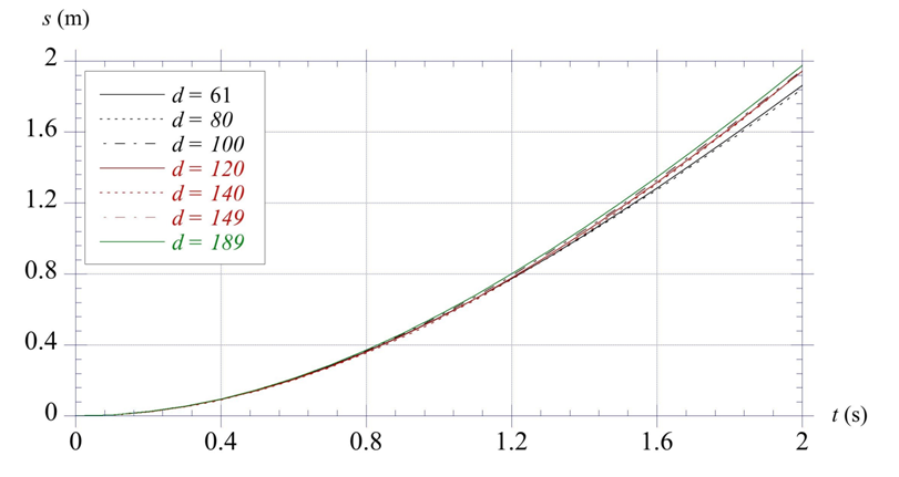
Fig. 2.5: Wave generation by underwater 3D slide. Experimental slide kinematics, as a function of initial submergence depth d , calculated with Eqs. (1-2 for Benchmark #1, 4) using average experimentally fitted values of S₀ and t₀ from Table 2.1.

Experiments were performed for 7 initial submergence depths d, which are listed in Table 2.1, together with values of related slide parameters and some measured tsunami waves characteristics. [Note the slight difference between the actual measured value of x_g and the theoretical value, due to experimental variance.] Regarding tsunami wave elevations, Table 2.1 lists, for each case, the measured characteristic tsunami amplitude η₀ (maximum depression at gage g1) and maximum runup on the tank axis R_u. Note, these small runup values were measured using a small digital camera directly viewing the waterline motion over a graduated scale. One should be cautioned that runup values might have been slightly affected by effects of the slide guiding rail.

Each experiment was repeated twice and both the raw and average time series of surface elevations measured at gages g1-g4 (t, η(t)) are provided as data files, for each experimental case in Table 2.1. Because raw measurements of slide kinematics were significantly processed in order to curve-fit the hydrodynamic coefficients of Table 2.1 corresponding to each experiment (i.e., average of 2 replicates), raw kinematics data is not provided here, but instead the curve-fitted coefficients that allow to recreate it in a numerical model, based on slide geometry and Eqs. (1-2 for Benchmark #1, 4) are given in Table 2.1, as well as data file with the average slide kinematics (t, S(t)).

Data:

Specifically, seven data files are provided (in both .txt and .xls format), which contain, for each of the 7 initial submergence depths (d = 61, 80, 100, 120, 140, 149, 189 mm), the time series of surface elevation measured at up to the 4 gages (in mm) listed g1, g2, g3, g4. In each file, when available, results are provided for each of two experimental replicates (or runs, marked as "r1" or "r2"), done for the same initial slide parameters, and for their average (marked as "ave"). In some of these tests, some data was missing for one of the runs and/or for one of the gages. In the latter case, this is identified in the name tag given each file. For instance, "d61g1234" (.txt or .xls), indicates that these are results for depth d = 61 mm and gages g1, g2, g3, and g4. Finally, data files are all provided as tab-delimited text files (with one line of title to skip) and excel spreadsheets. Fig. 9 shows all surface elevations available at gages for each experiment Solid curves are plotted for the average of 2 replicates and symbols denote partial raw data for each replicate.

Then, for each experimental case, we provide data files containing the average kinematics (kinematics.txt or kinematics.xls), (t, S(t)), recalculated for each average experiment, using Eq. (1-2 for Benchmark #1) and the values of S₀ and t₀ listed in Table 2.1 (calculated using Eqs. (4) and the other data in the table). As indicated before, Figure 2.5 shows a plot of the same data as given in these files; we see that the average kinematics is nearly identical for all the tests, up to 1.2 s or so. For later times, small differences in kinematics arise due to the experimental variability of the slide motion down the slope.

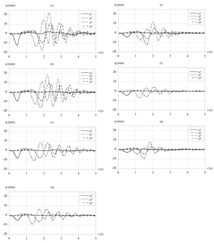
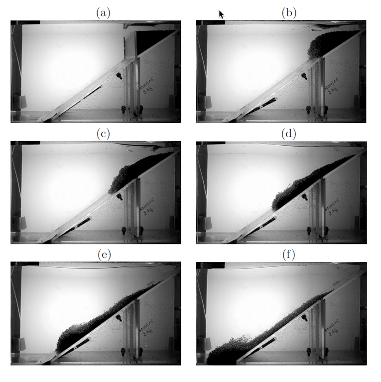
Fig. 2.6: Surface elevation measured at gages (g1, g2, g3, g4) in 3D submarine slide experiments. Symbols (o) and (△) denote experimental runs r1 and r2, respectively (only 1% of data points are shown), and lines denote their average. Initial slide submergence is as listed in Table 2.1, d = (a) 61, (b) 80, (c) 100, (d) 120, (e) 140, (f) 149, (g) 189 mm (see Figure 2.1).

Benchmark Problem:

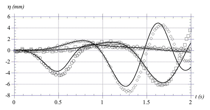
Fig. 2.7: Comparison of FNPF model results (-) with 3D submarine slide experiments of Enet and Grilli (2007) (symbols) for d = 0.140 m, at gage g1 (◇) and g2 (□) (only 10% of experimental data points are shown). [from Grilli et al., 2010].

The benchmark test here consists of using the above information on slide shape, density, submergence and kinematics (Table 2.1 and Figure 2.5), together with reproducing the experimental set-up to simulate surface elevations measured at the 4 wave gages (average of 2 replicates of experiments), such as shown in Figure 2.6, and present comparisons of model with experimental results, similar to Figure 2.7. We request that participants provide results for the cases with initial depth of submergence d=61mm and d=120mm.