Benchmark Problem #3: Three-dimensional submarine/subaerial triangular solid block

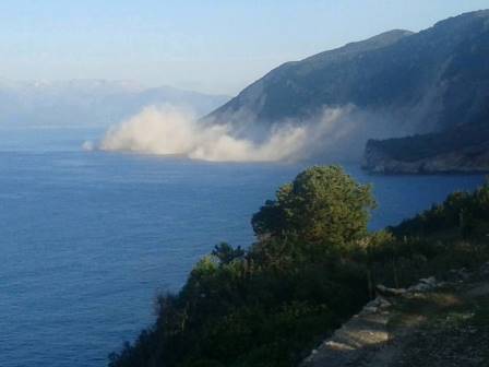
This benchmark problem is based on the 3D laboratory experiments of Wu (2004) and Liu et al. (2005) , for a series of triangular blocks of various aspect ratios moving down a plane slope into water from a dry (subaerial) or wet (submarine) location. See Figure 3.1 for pictures and Figure 2.2 for a sketch of experiments.

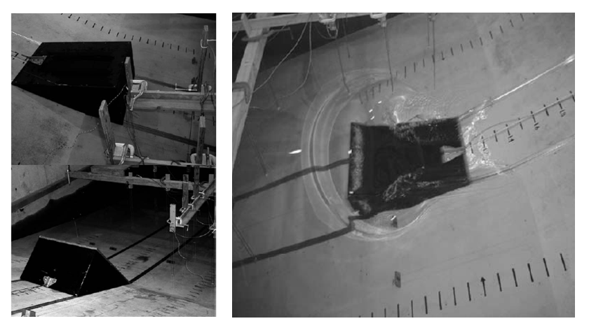
Fig. 3.1: Pictures of experimental set-up for 3D experiments of subaerial slides represented by triangular solid blocks. [from Liu et al., 2005]

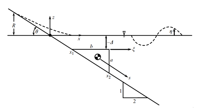
Fig. 3.2: Definition sketch for 3D experiments of submerged/subaerial (Δ</>0) slides modeled by triangular solid blocks moving down a plane 1:2 slope. [from Liu et al., 2005]

The experiments were conducted in a wave tank at Oregon State University (OSU), of length 104 m, width 3.7 m and depth 4.6 m. A plane slope 1:2 (Figure 2.2), i.e., with θ = 26.6 deg., was located near one end of the tank and a dissipating beach at the other end. In all the experiments, the water depth was h₀ = 2.44 m. While a few solid block shapes were tested, here, we only consider the experiments performed with a triangular block of length b = 0.91 m, width w = 0.61 m, (vertical) front face a = b/2 = 0.455 m (Figure 3.1, upper left and right; Figure 3.2), and mass M_b = 190.96 to 475.5 Kg. Hence slide volume is V_b = 0.126285 m³ and density, ρ_b = 1,512 to 3,765 Kg/m³ (note, the specific weight indicated in Liu et al. for the largest mass is, γ = ρ_b/ρ_w = 3.43, implying a slightly lower maximum density). Upon release, the slide model rolled down the slope on low-friction V-shaped wheels, about 3 mm above the slope, with its motion being recorded. The Coulomb friction coefficient measured in experiments for this block was C_n = 0.1577 to 0.2182, depending on block mass (see Table 1 in Liu et al.).

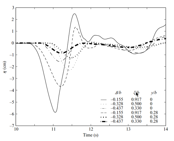
Fig. 3.3: Time histories of free-surface elevations measured at gages located at x/b = 1.20 and y/b (legend), for three initial slide submergences Δ/b. [from Liu et al., 2005]

In experiments, besides slide motion, the free surface elevation was measured at a few wave gages and the runup/rundown recorded on the slope. Figure 3.3 shows time histories of free-surface elevations measured at 2 wave gages located at x/b = 1.20 and y/b = 0 or 0.28 (see legend), for three initial slide submergences Δ/b = -0.155, -0.328, -0.437. For such submarine slides, Liu et al. defined their solid block acceleration a₀ with an equation identical to the first Eq. (4 for Benchmark #2). For subaerial slides, however, the equation simplified to a₀ = g sin θ (1 - tanψ/tanθ); this equations was used to compute the Coulomb friction coefficients listed in Table 1. Other similar results of experiments reported in Liu et al. are shown in Figure 3.4 and Figure 3.5 for Δ = 0.454 m (subaerial) and γ = 3.24 or 3.43.

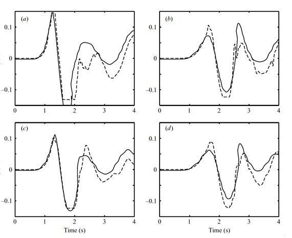
Fig. 3.4: Solid triangular block experiments for Δ = 0.454 m (subaerial) and γ =3.24. Computed (-) and measured (- - -) surface elevations at wave gauges located at (x, y) in m: (a) 1.83, 0; (b) 2.74, 0; (c) 1.83, 0.635; (d) 2.74, 0.635.

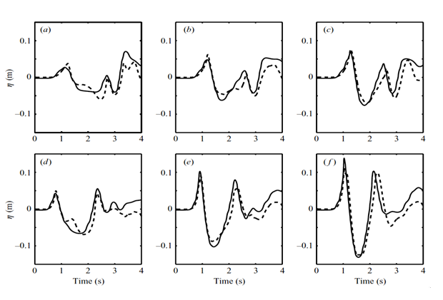
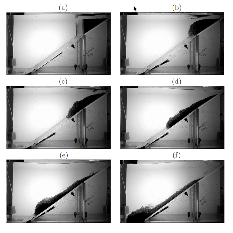
Fig. 3.5: Solid triangular block experiments for Δ = 0.454 m (subaerial) and γ =3.43. Computed (-) and measured (- - -) surface elevations at wave gauges located at (x, y) in m: (a) 0.4826, 1.092; (b) 0.8636, 1.092; (c) 1.2446, 1.092; (d) 0.4826, 0.635; (e) 0.8636, 0.635; (f) 1.2446, 0.635.

Wu (2004) and Liu et al. (2005) performed 3D-LES simulations, using the PLIC-VOF method and compared numerical results to their experimental data; some of these results are shown in Figure 3.4 and Figure 3.5. They prescribed the slide motion in the model, based on the measured slide displacement; see Wu (2004) for information on slide motions and details of numerical simulations. Abadie et al. (2010) simulated one of these subaerial slide case for Δ = 0.10 m (subaerial) and γ = 2.14 (Figure 3.5). They used a multi-fluid Navier-Stokes (NS) model, in which the solid slide was modeled as a fluid of very large viscosity and thus slide motion was implicitly computed as part of the solution (see Abadie et al. for results). Like Liu et al.'s simulations, Abadie et al.'s results for slide motion and surface elevations at gages (x/b = 2.001 and y/b = 0 and 0.694; Figure 3.6) were in good agreement with experiments, here without forcing slide motion.

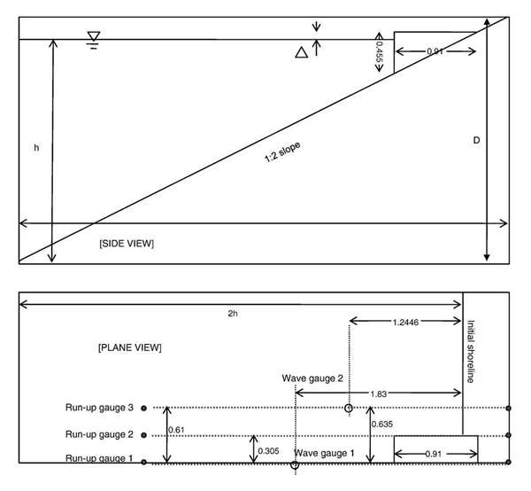
Fig. 3.6: Sketch of numerical simulation by Abadie et al. (2010) of one of Wu's (2004) and Liu et al.'s (2005) solid block experiments, with Δ = 0.10 m (subaerial) and γ = 2.14.

Data:

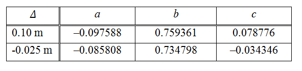
Data is provided (recorded block motion, wave gage and runup measurements for the two different initial elevations of the wedge on the beach. The recorded block motions were curve-fitted as a function of time t, giving the horizontal distance, x_0,t= x_0,t=0+(at³+b²+ct)cosβ, where β = arctan(1/2) and x_0,t=0 = -2Δ. The polynomials' coefficients have been determined as follows for both cases:

Measured free surface elevations are given for each case, for 2 wave gages placed at: (x,y) = (1.83, 0) and (x,y) = (1.2446, 0.635) m, where x = distance to the initial shoreline, y = distance to the central cross-section (Figure 3.6). Measured runup is given for each case, at runup gages 2 and 3 (Figure 3.6), lying on the slope at distance 0.305, and 0.61 m from the central cross-section.

Data is given in separate text files, in meter, as time versus elevation (t, η); files are named benchGG02-X_wave_gage_Y.txt and benchGG02-X_runup_gages_Y.txt, where X is the run number (30 for the first case and 32 for the second case), and Y is the gage number (1 or 2 for the wave gages and 2 or 3 for the runup).

Problem:

The benchmark here consists in using the above information for the solid wedge sliding down the 1:2 slope, and details in references, to reproduce the experimental set-up (see Figure 3.6) and simulate surface elevations measured at the wave gages and runup/rundown measured on the beach for two initial locations of the block, with: Δ = 0.1 m (subaerial); and Δ = -0.025 m (submerged). As a minimum results should be provided for the same experiment as in Abadie et al. (2010) with Δ = 0.1 m.