TEST OF MEANS

1. AGENDA:
1. Test of a mean.
2. Overview
1. Sampling distribution: standard normal
2. Critical values and regions
3. One-tailed and two-tailed tests
3. Reading:
1. Agresti and Finlay, Statistical Methods, Chapter 6:
1. Read pages 155 to 159 for general ideas regarding hypothesis testing.
2. Read pages 1159 to 167 for test of the mean procedures.



2. ANOTHER EXAMPLE OF THE BINOMIAL:
1. This section repeats the notes from Class 23.
2. Problem: a population of available jurors in a city contains 53 percent of the population who do not favor capital punishment. This is known from a detailed public opinion survey. A local judge is suspected of approving only potential jurors who favor the death penalty. The last jury consisting of 12 people which dealt with a murder case contained only 5 people who said they opposed capital punishment. Is there any evidence of selective bias?
3. Hypotheses:
1. The "research" hypothesis is that the judge is biased which means that the proportion of "anti-capital punishment jurors" will be less than .53. Thus, the H_A (H_A is the alternative hypothesis.)
2. The null hypothesis is P =.53.
1. The H₀ asserts that a population parameter equals a specific value.
3. Since the alternative hypothesis (H_A) is that P is less than .53 we will consider only those sample results at the "low" end of the scale as disconfirming evidence. This is a one-tailed test of significance. (See below.)
4. Sampling distribution and critical region:
1. Let us decide ahead of time that we will consider any sample result that occurs with probability less than .02 as evidence that the null hypothesis should not be accepted.
2. The sampling distribution and critical region and critical values for this problem are shown in the figure on the next page. Note that N = 12 and P = .53:

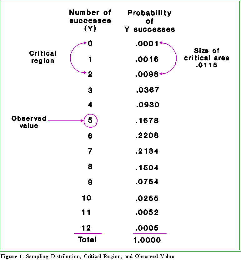
1. Given the nature of the problem, we will reject the null hypothesis only if we get, say, 0 or 1 or 2 "anti-capital punishment" jurors; that is, we will use only one tail of the sampling distribution to test the hypothesis.
2. Sometimes when there is no clear alternative hypothesis we will consider unlikely events at both ends of the distribution.

1. Critical value: we have agreed ahead of time to reject the H₀ if a sample result occurs with probability of .02 or less. Thus, from the above distribution we see that the critical region includes outcomes 0, 1, and 2. The outcome 3 occurs with probability .0367 and is therefore above the critical value.
2. Hence the decision rule is: reject H₀ if and only if Y, the number of "successes," is 2 or less.
1. The level of significance is therefore .02.
3. Sample result: the data indicate that Y = 5 jurors oppose capital punishment. The sample result is thus 5 which we compare with the critical value.
4. Decision: since 5 is greater than 2 (the critical value) we do not reject the null hypothesis.
5. Interpretation: We have concluded that the judge is not biased against jurors who oppose the death penalty. There is a chance that we have made a mistake, but this time the possible error is in failing to reject a null hypothesis that should be rejected.



1. THE TEST OF A MEAN - OVERVIEW:
1. The hypothesis is that , the population mean, equals a specific value.
2. This is a large sample test: N must be at least 75 or larger.
3. The sampling distribution is the standard normal
1. That is, sample statistics will be converted to standard scores (you have already done this) and compared to a standard normal critical value
4. The standard deviation of the sampling distribution is called the standard error of the mean. It is often denoted .
5. In effect, we will calculate a sample z and compare it with a critical z.
6. Review:
1. You should review the material pertaining to the standard normal distribution, the mean, and the standard deviation.
2. Reviewing these notes on your own may also be helpful. This material is not at first sight obvious but with a little work it can be mastered.



2. LARGE SAMPLE TEST OF MEAN:
1. Problem: George Easterbrook writes: "Farm families as a group are not poor. Their average income in 1983, one of the worst years in memory for agriculture, was $21,907." Yet a sample of 100 tax returns from farm families across the country shows the average family income to be $18,900 with a standard deviation of $1,000. Given that you have a great deal of confidence in the independence of the sample, the data support Easterbrook's contention that farm family income is $21,907?
2. Assumptions and requirements: we assume that the sample is SRS and that there are at least 75 cases. (In this problem that requirement is met because N = 100.) If the sample is less than 75 another procedure is used, as we will discuss in a coming class.
3. Hypotheses:
1. The research hypothesis (H_A)is that m is less than $21,907 because we suspect that the stated value is too high.
1. That is, H_A: m < $21,907
2. The null hypothesis (H₀) is, however, m = $21,907.
4. Sampling Distribution:
1. If repeated samples of size N are drawn from a population having a mean and variance s², then as N becomes large the sampling distribution of the sample means, , becomes normal with mean and standard deviation . (The standard deviation of the sampling distribution is called the standard error of the mean. See below.)
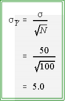
2. In words, suppose we take a sample of size N = 100 from a population with a mean of m = 500 and standard deviation of s = 50. Using these 100 cases we calculate the mean (average) of the data with the usual formula. (That is we calculate the for this particular sample.) Now suppose we obtain a second, independent sample of 100 and do the same thing; that is, get a second Then we repeat the process another time and another and another...each time calculating a sample mean If we kept on doing this thousands and thousands of times what would the collection of sample means look like? How would they be distributed? What would a stem-and-leaf display show? What would the mean of the means be?
1. The answer, given by statistical theory, is that these means would have a normal distribution, the mean of which would be the population mean (m = 500 in this case), but the standard deviation would be not sigma, the population standard deviation, but rather sigma divided by the square root of N. The standard deviation of the sample means would be:

1. Figure 2 on the next page shows a general picture of the theoretical sampling distribution.

1. The distribution of sample means is normal with a standard deviation (called the standard error of the mean or simply the standard error) equal to sigma divided by the square root of N.
1. Thus, if we are dealing with sample means based on relatively large N's (more than 75) the appropriate sampling distribution is the normal distribution.
2. Remember, a sampling distribution is used to show the probability of obtaining a particular sample result or one even more unlikely. Knowing that sample means have a normal distribution allows us to use our knowledge of the normal distribution to make inferences about the likelihood of a particular sample mean occurring, given that the hypothesized population mean is such and such.
3. Furthermore, we found that we can always convert raw data to standardized data so that we can use a "tabulated" standard normal distribution. (See below.)
2. In the present problem, the hypothesized population mean is $21,907 whereas the sample mean is $18,900. Using the standardized normal distribution as the sampling distribution allows us to say whether the sample result could have arisen by chance (given the null hypothesis) or whether it is such an unlikely event that we want to reject the null hypothesis.
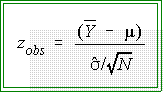
3. To use the standard normal distribution one must convert raw data--here the sample mean--to a standardized or z score.
1. The formula for doing so is this:

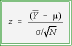
1. To use this formula one has to know s, the population standard deviation which is unknown so we estimate it by using, the sample standard deviation. Now the formula for getting an observed z is:

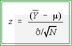
1. The quantity, is called the standard error of the mean. It is interpreted as the standard deviation of the sampling distribution of the mean.
1. Before leaving the topic let's look at the standard error of the mean a bit more.
2. Suppose sigma, the population standard deviation, equals 100 and N is relatively small, say 10. Then if we take repeated samples of size N = 10, calculate a each time, and plot the result we will get a figure that looks something like the previous figure.
3. Now suppose we do the same thing--take repeated samples and get sample means but this time use much larger sample sizes, say N = 100. The result would be a normal distribution with mean , but a smaller standard deviation.
4. What is going on is this: each time we take a sample from a population with a mean of and s = 100 and calculate the observed sample mean will not equally exactly the "true" value because of sampling error. Sometimes be too large, sometimes it will be too small, and only very, very rarely will it equal the true value. But over the long run, the average of the averages, so to speak, will equal the population mean. Hence, we say the expected value of sample means, equals the population mean, m . In symbols,

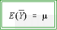
1. This is read as "the expected (long run) value of sample means equals the population mean from which the samples are drawn.
1. Note in addition this important fact, which may be intuitively clear: as the sample sizes get larger and larger, the sample means should come closer and closer to the true value, although in most instances they will not equal it. That is, if you have a sample of 5, your sample may be quite far from the true value, but if you increase your sample to 1,000 then the will in all likelihood be quite close to the true value. This idea is reflected in the standard errors of the sampling distributions: when N is only 5 the tend to be scattered widely above and below the true value, but when N is 1000 the (which are guesses) about the true value tend to be bunched close together. You can have more "confidence" in a sample mean based on 1000 cases than on one based on just 5 observations. But note:

holds no matter what the sample size. In other words, small samples are just as "valid" as large ones--their expected values equal the true parameters--but they do not give you as much confidence because any particular value of a small sample might be quite far from the true mean.

1. Look carefully at the formula for the standard error and you can see this concept even more clearly: for a given sigma (the population standard deviation) as N increases the denominator of the formula increases and the standard error decreases. Here are a few examples:

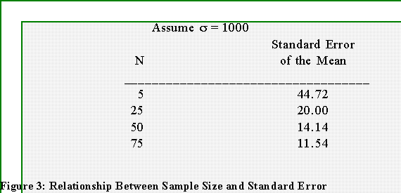
1. We see that as N increases the standard deviation of the sampling distribution (called, remember, the standard error) decreases. This makes sense because the variability of sample estimates of should be less when the sample is based on 1,000 or 10,000 cases.
1. Level of significance and critical region:
1. Suppose we want the level of significance to be .05. The level of significance, you will recall, is the probability of making a Type I error--of incorrectly rejecting the null hypothesis.
2. Our job then is to find a critical value which will define a critical region of such a size that the probability of falling into it is .05, given of course that the null hypothesis is true.
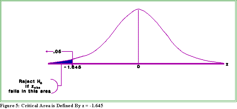
3. Since we are dealing with a normal distribution, however, we know how to find values that mark off various portions of the curve or distribution. Consider the familiar picture:

1. To find the critical value, locate the z from the table of the standard normal that corresponds to .5 - .05 = .45. It is about 1.645. Since we are looking at the left side of the curve the critical value is actually minus 1.645.
1. Figure 5 shows the idea:

1. The question is now: does the sample mean ($18,900) when converted to a standardized z score fall into the critical region. That is, is the observed z based ongreater than or equal to the absolute value of the critical z? If so, reject the null hypothesis; if not accept it.
1. Test statistic:
1. To calculate the test statistic convert the observed($18,900) to a standard score. You know how to do this except that since we are dealing with a sampling distribution we use the standard error, denoted, instead of the standard deviation. The formula is:

1. For this problem the observed z is:

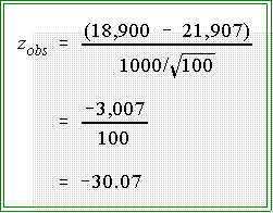
1. The observed z is thus -30.07
1. Decision:
1. Since the absolute value of the observed z is very much greater than the absolute value of the critical z we reject the null hypothesis.
2. Interpretation:
1. It appears that the Easterbrook's assertion about farm income is incorrect: in fact, it may be much less than he suggests.
2. Given that we have not accepted the H₀ our best estimate of the true value is now $18,900.
3. After rejecting a null hypothesis, you should try to make an estimate of what the true value is. In the case of sample means, the value is an "unbiased" estimator of m.



1. NEXT TIME:
1. More on tests of means and proportions.

Go to Statistics main page

Go to H. T. Reynolds page.

Copyright © 1997 H. T. Reynolds