DEPARTMENT OF POLITICAL SCIENCE
AND
INTERNATIONAL AFFAIRS
Posc/Uapp 815
STATISTICAL INFERENCE

- AGENDA:
- Basic ideas of statistical inference.
- Sampling distributions
- Critical values and regions
- Types of errors in making inferences
- Reading:
- Agresti and Finlay, Statistical Methods,
Chapter 6, pages 154 to 167.
- INFERENCE:
- This section repeats the notes from the last class.
- Goals of statistical inference:
- Test hypotheses about population parameters
- Estimate the magnitude or value of population parameters
- A simple example:
- Question (hypothesis): Suppose you are flipping coins with someone. A
reasonable question is: is the person honest?
- How should one "operationalize" the notion of honesty?
- The question really asks: is the probability of getting a "head" on a single
flip of a coin 1/2 = .5? The hypothesis suggested by the question, in other
words, is that P[heads] = .5 More formally,

- H0 is called a null hypothesis
- In a series of , say, 10 flips of a coin
how likely is it that a person will get 9
heads?
- In order to answer this question you have to decide two things:
- What is "likely"? That is, what is your definition of likely or
probable and conversely what is your definition of improbable?
- Given this definition, you then have to decide what outcomes--what
number of heads in 10 tosses--that you will consider probable and
what number you will believe to be improbable.
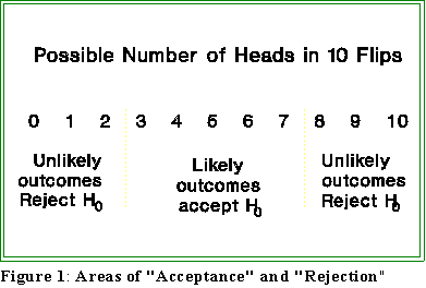
- Stated another way you have to form a mental picture like this:

- Next, observe an actual set of ten tosses and count the number of heads.
- Finally, make a decision using the guidelines presented above: if the
observed number of heads fall in the region of rejection because this result
is improbable, then reject the hypothesis (P [heads] = .5) and conclude that
the coin is biased, the person is crooked, etc.
- If, for example, someone tosses a coin 10 times and obtain 9 heads then
you might suspect that the hypothesis of honesty is untenable.
- STEPS IN TESTING A HYPOTHESIS:
- Problem: A drug manufacturer claims that its anticoagulant drug is 80 percent
effective (that is, the probability of preventing clots is .8) based on thousands of
trials with primates, mice, and even human volunteers. The FDA has sent you data
pertaining to 8 randomly selected individuals in a Veterans hospital, only 2 of
whom were helped by the drug. If the "true" proportion of "success" is .8, how
likely is it that you would observe only 2 out of 8 successes? Could this result have
occurred by chance, thereby supporting the manufacturer's claim or is it such an
improbable result that you are led to doubt the drug's efficacy?
- Research hypothesis: The FDA believes that the probability of success is less than
.8 (that is, P < .8).
- The null hypothesis is: H0 = .8
- A null hypothesis always asserts that a population parameter equals a
specific number, frequently zero but in this case .8.
- Sampling Distribution:
- Loosely speaking, a sampling distribution is a theoretical distribution that
shows the relationship between the possible values of a given sample
statistic (e.g., sample number of successes) based on N cases and the
probability associated with each possible value.
- Thus, if we know a sampling distribution for a statistic, if we have a sample
of N cases, if we have an actual observed value of the statistic, and if we
have a particular null hypothesis in mind, we can tell how likely the
observed result is. Based on this information, we can decide whether or not
to accept the null hypothesis.
- In this case the statistic in question is simply Y, the number of successful
treatments in N trials.
- Hence, in this case we have N = 8 and have observed Y = 2.
- An appropriate sampling distribution will tell us the likelihood of getting 2
or fewer successes in 8 independent trials given that the null hypothesis is
true.
- The material that follows is designed to show where this particular sampling
distribution comes from.
- To find the probability of Y successes in N trials given that the probability
of success is P use this formula:

- The term P(Y,N,P) means the "probability of getting Y successes in N
trials given that the probability of success is P.
- As we have already seen, the symbols N! and Y! mean "factorial"
N! = N(N - 1)(N -2)(N -3)....For example, 8! = (8)(7)(6)...
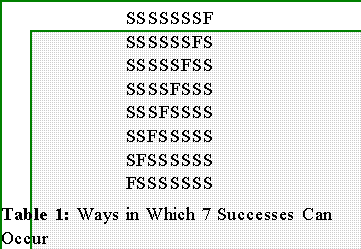
- The first part of the equation represents how many ways Y
successes can be obtained in 8 trials. For example, these are the
ways we can obtain 7 successes in 8 trials:

- In the table S denotes a success and F a failure. In the first line, 7
successes are obtained on the first 7 trials. But this is not the only
way to get seven successes. The second line shows, for example.
that 7 successes can be obtained by getting 6 in a row, then a
failure, then another success.
- The number of these patterns is given by the first part of the equation; that
is,

- The second part of the equation gives the probability of getting Y
successes in N trials if the probability of success is P. This probability must
be multiplied by the number of ways of getting Y successes (see above).
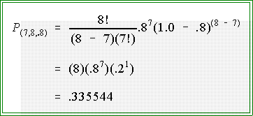
- Example: suppose the probability of getting a "success" is P = .8. In addition,
suppose we want to know the probability of getting Y = 7 successes in N = 8 trials
or attempts. According to the formula the probability is

- Note that 8! = (8)(7)(6)(5)(4)(3)(2)(1); that 7! = (7)(6)(5)(4)(3)(2)(1); and
that 1! = (1). Thus, the first part of the equation reduces to 8, since 8!/7! =
8 which in turn is divided by 1. See the listing above.
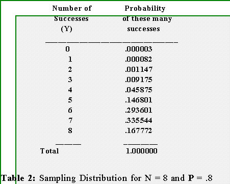
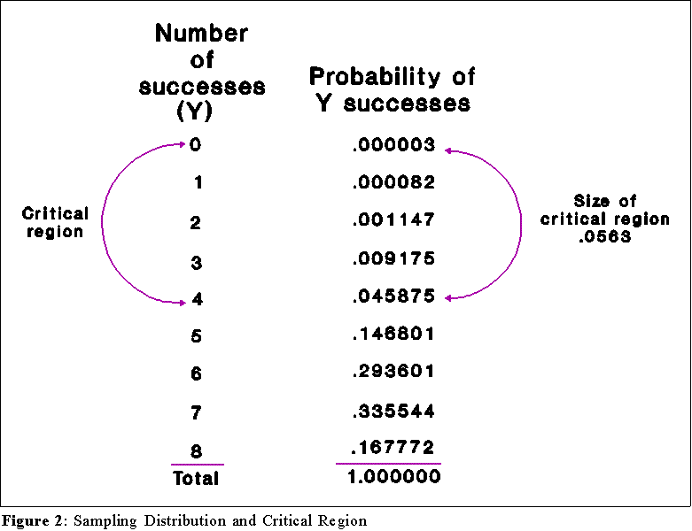
- By letting N = 8, P = .8, (1 - P) = .2, and letting Y equal successively 0, 1,
2, 3,...we get this sampling distribution.

- You can get this table from MINITAB by opening the session window and typing
at the MTB> prompt

- Parts of the Sampling distribution
- Decide which sample outcomes (e.g., number of successes) are so
improbable to you that should one of them occur, you will not accept the
null hypothesis. This is called the critical region.
- The cutoff value--the value at or below which you reject the null
hypothesis--is called the critical value.
- In this case let it be 4: hence if you observe 4 or fewer successes in
8 trials you will reject the H0 that the true probability of success is
.8.
- Now also realize that whenever you make a judgment of this sort you run the risk
of making an error because you are, in effect, saying that a result is "improbable"
but not "impossible." There is therefore a probability, however small you wish to
make it, that you have made an incorrect decision. Why? Because the critical
region contains values that could occur but are so unlikely that you believe that
they did not arise under the null hypothesis.
- This kind of a mistake is called a Type I error and the probability of making
it is the probability of falling in the critical region.
- This probability, usually denoted by ,is also called the level of
significance.
- Here is the sampling distribution again.
Let us define the values of Y 0, 1,
2, 3, and 4 as the critical region. (See the figure below.)

- To summarize:
- Critical region: those possible sample results that will cause us to
reject H0 if one should actually occur.
- Critical value: if an observed sample value exceeds this we will
reject H0. The critical value is thus the demarcation point between
the critical region and the region of acceptability.
- Type I error: rejecting the H0 when it is true.
- The level of significance is another term for the probability of
making a Type I error.
- Collect data and compute sample statistic:
- Here the job is particularly easy: Y is 2 out of 8.
- Decision:
- Compare the sample statistic to the critical value: if it is greater than the
critical value (in this case) accept the null hypothesis; if is equal to or less
than (in this case) the critical value reject H0.
- Interpretation:
- Here we reject the null hypothesis because the observed Y of 2 is less than
4, the critical value.
- There is a small chance that we have incorrectly rejected H0 because the
probability of observing 2 or fewer successes given that P equals .8 is the
sum of the probabilities associated with 0, 1 and 2 successes. It's not a
large chance but it is a chance.
- If we falsely reject the null hypothesis, we are in effect telling the FDA to
ban the drug when in fact it might help many people. Given that knowledge
we might want to make the level of significance even lower--that is we
might want to minimize the chance of Type I error even more.
- ANOTHER EXAMPLE OF THE BINOMIAL:
- Problem: a population of available jurors in a city contains 53 percent of the
population who do not favor capital punishment. This is known from a detailed
public opinion survey. A local judge is suspected of approving only potential jurors
who favor the death penalty. The last jury consisting of 12 people which dealt with
a murder case contained only 5 people who said they opposed capital punishment.
Is there any evidence of selective bias?
- Hypotheses:
- The "research" hypothesis is that the judge is biased which means that the
proportion of "anti-capital punishment jurors" will be less than .53. Thus,
the HA (HA is the alternative hypothesis.)
- The null hypothesis is P =.53.
- The H0 asserts that a population parameter equals a specific value.
- Since the alternative hypothesis (HA) is that P is less than .53 we will
consider only those sample results at the "low" end of the scale as
disconfirming evidence. This is a one-tailed test of significance. (See
below.)
- Sampling distribution and critical region:
- Let us decide ahead of time that we will consider any sample result
that occurs with probability less than .02 as evidence that the null
hypothesis should not be accepted.
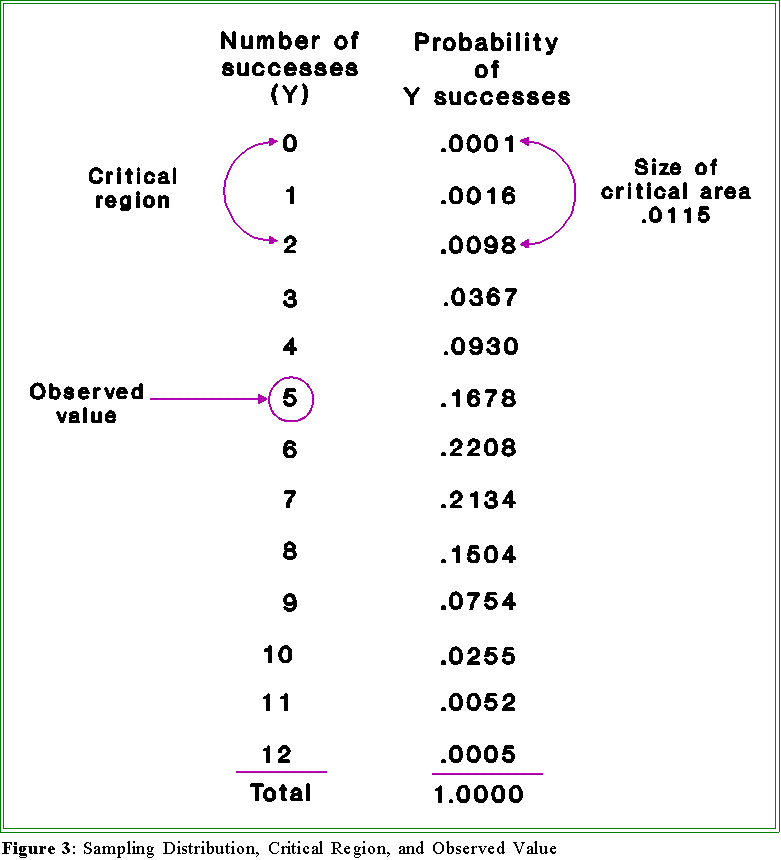
- The sampling distribution and critical region and critical values for
this problem are shown in the figure on the next page. Note that N
= 12 and P = .53:

- Given the nature of the problem, we will reject the null hypothesis only if
we get, say, 0 or 1 or 2 "anti-capital punishment" jurors; that is, we will
use only one tail of the sampling distribution to test the hypothesis.
- Sometimes when there is no clear alternative hypothesis we will consider
unlikely events at both ends of the distribution.
- Critical value: we have agreed ahead of time to reject the H0 if a sample
result occurs with probability of .02 or less. Thus, from the above
distribution we see that the critical region includes outcomes 0, 1, and 2.
The outcome 3 occurs with probability .0367 and is therefore above the
critical value.
- Hence the decision rule is: reject H0 if and only if Y, the number of
"successes," is 2 or less.
- The level of significance is therefore .02.
- Sample result: the data indicate that Y = 5 jurors oppose capital
punishment. The sample result is thus 5 which we compare with the
critical value.
- Decision: since 5 is greater than 2 (the critical value) we do not reject the
null hypothesis.
- Interpretation: We have concluded that the judge is not biased against
jurors who oppose the death penalty. There is a chance that we have made
a mistake, but this time the possible error is in failing to reject a null
hypothesis that should be rejected.
- TYPES OF ERRORS IN HYPOTHESIS TESTING:
- Here are the two types of errors one can make in statistical inference:
- Type I: Rejecting a null hypothesis that is really true.
- The probability of making this type of error, under the assumptions
and conditions mentioned above, is a.
- One can interpret in various ways:
- It is the "size" of the critical region. If the null hypothesis,
H0, is really true, then a critical region of size is the
probability that a sample result will lead to an incorrect
decision. That is, the sample result, since it falls in the
critical region, will suggest that we reject H0, when it should
not be.
- a is called the level of significance.
If, for example, we use
an a of .05,
and the sample result falls in the critical region,
we say that the result is "significant at the .05 level." If a
is .001, and the sample result still falls in the critical region we
say it is "significant at the .001 level."
- Keep in mind, however, that is the probability of
making a type I error, which is to incorrectly or falsely
reject a "true" null hypothesis.
- Type II: Failing to reject a hypothesis that is really false.
- The probability of incorrectly accepting a false H0
is b. It is not
exactly the opposite of since its size depends on how false the
null hypothesis is.
- The power of a test: the power of a
statistical test is defined as 1 - b.
It tells one the chance of detecting a false H0.
- NEXT TIME:
- Tests of means and proportions.

 Go to Statistics main page
 Go
to H. T. Reynolds page.
Copyright © 1997 H. T. Reynolds

