Excel 7: A Tipsheet

Contents

• Description
• Starting Excel
• Creating a worksheet
• Editing a worksheet
• Working with formulas
• Sample calculations
• Getting online help
  

Description

Excel 7 is a spreadsheet program for use with Windows 95. It is a flexible tool for performing simple or complex calculations, and can be used to create tables, graphs, or charts. This tipsheet provides basic information for getting started using Excel 7. Since other versions of Excel have the same features, the instructions in this tipsheet also should apply to those versions.

Contents Help

Starting Excel

1. Click on the Start button to open the Windows 95 menu.
2. Select "Programs".
3. Select "Microsoft Excel".

Position the mouse pointer over any button to display the name of the button.

You can get Help by clicking on the Help button in the top-right corner of the screen, then clicking on a part of the screen, menu, or any button with which you need help. You can also access online help using the "Help" menu or by pressing the F1 key. (Under the "Help" menu, the Lotus 1-2-3 Help command will show you the Excel equivalents for the Lotus 1-2-3 menu and command items.)

Exit Excel by (1) selecting the "File" menu, then choosing the Exit command (2) clicking the Program Close button in the upper-right corner of the Excel window, or (3) pressing the Alt-F4 key combination.

Contents Help

Creating a worksheet

Each Excel file constitutes one workbook. Initially, a workbook is made up of 16 worksheets (you can add or delete sheets as needed). You can use the scrolling buttons (the arrow buttons located at the bottom-left corner of the screen) to move around a workbook and those at the bottom-right to move around a worksheet.

The active cell is the highlighted cell. Clicking on any cell will activate that cell.

Methods for selecting several cells:

• Click on the first cell and drag through to the last cell.
• Click on the first cell; hold down the SHIFT key and click on the last cell to select all cells in between.
• Hold down the CTRL key and click on each cell you want to select.

Pressing ENTER will change the active cell within the selected cells. Pressing the SHIFT-ENTER key combination moves the active cell backward. Pressing the TAB key moves the active cell from left to right, and pressing the SHIFT-TAB key combination moves the active cell from right to left.

Entering data: Excel displays data in both the active cell and in the Formula Bar above the worksheet. You can enter or modify data in the cell or the Formula Bar. Three buttons (Cancel, Enter, and Function Wizard) also appear in the Formula bar. The Cancel button cancels the entry and removes it from the Formula bar and the active cell. The Enter button enters the data. You can also enter data using the directional arrows, TAB key, and ENTER key on the keyboard. The Function Wizard button displays a dialog box for choosing functions.

Changing cell contents: Select a cell. Position the pointer over the data in the Formula Bar. Click and drag over the data you wish to change. Type new data or erase existing data using the BACKSPACE key or the right mouse button (select "Cut"). Press ENTER.

You can also double-click on a cell, select the data in the cell, and enter new information. Press the HOME key to move the insertion point to the left of the data.

Widening a cell: Position the pointer between two columns so that the cursor changes to a two-directional arrow. Click and drag the mouse pointer to the right and release it. You can also double-click on the column border. The column width will adjust to fit the widest cell entry.

Undo/Redo : The Undo button (the left-pointing arrow) allows you to reverse your last action (or, press the CTRL-Z key combination). The Redo button (the right-pointing arrow) allows you to reverse the Undo command (or, press the CTRL-Y key combination). Press the ESC key to close the Undo list without making a selection.

Save: Save your workbook by clicking on the Save button . The first time you save a file, you must give it a name and identify to which disk and directory you want to save the file. The button below the Program Close button that is also marked with an X is the File Close button. The File Close button or the CTRL-F4 key combination will close a file and leave Excel open.

Contents Help

Editing a worksheet

Clearing cell contents: Use the DELETE key to clear the contents of a cell. To remove a cell's formatting, select "Clear" from the "Edit" menu, then choose All, Formats, Contents, or Notes from the submenu.

Inserting and deleting rows and columns: You can insert new rows or columns using the "Insert" menu (then choosing "Rows" or "Columns") or by clicking on the right mouse button and choosing insert or delete. New rows are inserted above the selected row. New columns are inserted to the left of the selected column.

Moving: To move the contents of a cell, select a cell or range of cells. Position the pointer on the gray border (the pointer becomes an arrow). Drag the outline to another location. Release the mouse button. Also, you can use the Cut, Copy and Paste buttons in the tool bar to move or copy the contents of a cell.

Copy: To copy the contents of a cell, select a cell or range of cells. Hold down the CTRL key and position the pointer on the gray border (the pointer becomes an arrow with a plus sign). Drag the outline to another location. Release the mouse button and the CTRL key to copy the cells. Also, you can use the Cut, Copy and Paste buttons in the tool bar to move or copy the contents of a cell.

Copy and Paste Shortcut Keys: Use the following procedure to copy the contents of an active cell to a non-adjacent cell:

1. Select the cell.
2. Press the CTRL-C key combination to place a copy of the formula in the Clipboard.
3. Select the cells to which you want the formula copied.
4. Hold down the CTRL key and press the left mouse button.
5. Press the CTRL-V key combination to paste a copy of the formula in the selected cells.
6. Press the ESC key.

Contents Help

Working with formulas

Using Autosum: Select the cell, then click on the Autosum button to create a formula. A flashing dotted line appears around the range of the cells that will be summed. Click the Autosum button again.

Building a simple formula:

1. Select the cell in which you want the formula.
2. Type an equal sign (=). Every formula must begin with an equal (=) sign.
3. Enter the cell reference and operands that tell which function to perform. Choose the cell references with your pointer by clicking on the cells you want included.
4. Click on the Enter box in the Formula Bar.

Using the fill handle: The fill handle is a small handle in the lower-right corner of the active cell.

To copy the contents of an active cell into adjacent cells, perform the following steps:

1. Select cell or range of cells.
2. Position the mouse pointer over the fill handle in the lower-right corner of the cell or range of cells. When you position the pointer over the fill handle it becomes a small plus sign (+).
3. Click and drag through all cells to which you wish to apply the formula.

You can also copy a formula to a range of cells by using the Edit, Fill, Right (CTRL-R key combination) or Edit, Fill, Down (CTRL-D key combination) commands.

Holding down the SHIFT key while using the fill handle will insert blank cells.

Dragging the fill handle into the active cell erases the contents of the active cell.

Using the Function Wizard: The Function Wizard provides step-by-step instructions for constructing complicated formulas that require more than one cell reference. Use the Function Wizard button in the Formula Bar to access the features.

Contents Help

Sample calculations

The following Excel samples -Using Excel to calculate averages and Using Excel to calculate a loan payment - use many of the features of Excel. The averaging example demonstrates how to create a formula in the formula bar, while the car loan example shows how to create a formula with the Function Wizard.

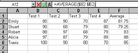
Using Excel to calculate averages: To find the average test scores for five students, follow these steps.

1. Open a new Excel worksheet.
2. In column A, beginning in row 2, type the names of five students.
3. In row 1, beginning in column B, type the headings Test 1, Test 2, Test 3, Test 4, and Average.
4. Type the test scores for each student in the appropriate cells, leaving the Average column empty. (Enter each score using the Tab or Enter key.)
5. Select cell F2 (the first cell to which the formula will be applied).
   
6. Click in the Formula Bar and type the following formula:
   
   =AVERAGE($B2:$E2)
   
   NOTE: The $ in the formula indicates an absolute reference; the colon indicates a range of cells.
   
   
7. Click the enter button. The average for the first student appears in cell F2.
8. Use the fill handle to drag the formula through column F. The average for each student appears in column F.
9. Save your worksheet. It should look like this:
   

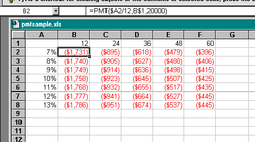
Using Excel to calculate a loan payment: You can use Excel to determine a variety of monthly payment plans for a $20000 car at a variety of interest rates.

1. Open a worksheet in Excel. Save it as "pmtplan.xls".
2. In column A, beginning in row 2, enter 7%, 8%, 9%, 10%, 11%, 12%, and 13% (the rates of available loans).
3. In row 1, beginning in Column B, enter 12, 24, 36, 48, and 60 (the number of months in available loans).
4. Select cell B2. Then, from the right mouse menu, select "Format Cells…". Choose "Currency", then set the Decimal Places to 0. Click OK.
5. Click the Formula bar to display the cancel, enter and function buttons. Click the Fx button.
6. From the Function Category box, choose "Financial." From the Function Name box, choose "PMT". Click Next.
7. In the rate box, type A2. Press the F4 key 3 times to make the cell reference absolute. Divide the rate by 12 months ($A2/12).
   
   Note: The F4 key lets you toggle through a variety of settings for the absolute identifier.
   
   
8. In the nper box, type B1. Press the F4 key twice to make the cell reference absolute (B$1).
9. In the present value (pv) box, type 20000 (the cost of the car).
10. Click Finish.
11. Click the enter button. The payment for a 12-month, 7% loan appears in cell B2.
12. Use the fill handle to drag the formula through the chart.
13. Save your worksheet. It should look like this:
    

Contents Help

Getting online help

You can get online help in one of the following ways:

1. Click on the Start button in the Taskbar, then click on the "Help" command. Review Using Windows 95 Help, which contains instructions for using the "Help" command.
2. Press the F1 key.
3. Click on the Help button in the Toolbar or select "Help" from the Menu Bar.
4. Download Excel tutorials from the Microsoft Home Page.

If you need help working with Excel 7.0, send e-mail to consult@udel.edu or call the IT Help Center at 831-6000.

Contents

Return to Microsoft Excel 7 cover page.

Technology Home Page
URL of this document: http://www.udel.edu/topics/software/general/spreadsheet/excel7/exceltips.htm

This page is maintained by Sigurd Andersen .

Last Modified: March 1997