For a collection of particles that do not interact, we recall that the ideal gas description is sufficient to predict properties of fluids at certain limiting conditions. Within such a description, the particles, of certain masses, are considered to be moving with velocities that are distributed in a certain fashion. We now consider this distribution of velocities, starting with the distribution of velocity in one-dimension. The generalization to three dimensions follows.
We are concered with finding a velocity distribution function. This mathematical description provides the probability of a particle having the Cartesian components of velocity in the range
![]() ,
,
![]() , and
, and
![]() .
.
We let the distribution function be:
With the definition of the probability density distribution above, we can determine the probability of a particle having
the components of velocity
![]() ,
,
![]() , and
, and
![]() as:
as:
An assumption regarding the nature of this distribution: the gas is isotropic such that the direction of particle movement does not affect the properties of the fluid. In this sense, the velocity distribution is effectively dependent on the magnitude of the velocity. The magnitude of the velocity is:
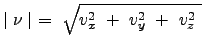 |
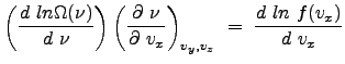
We now consider the natural logarithm of the distribution function:
with
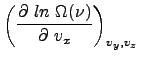
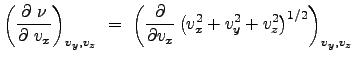
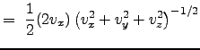
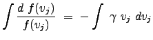
To determine ![]() , we consider the derivative of the probability function
, we consider the derivative of the probability function ![]() with respect to the variable
with respect to the variable ![]() .
.
 |
|||
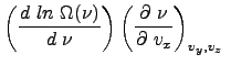 |
One can show that
 .
.
 |
|||
 |
|||
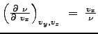
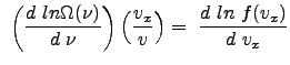
Using this last relation, we obtain:
 |
|||
 |
|||
 |
Since each direction is equivalent (under our assumption of isotropy of the medium), we can write for the ![]() and
and ![]() differentials (and
you can show yourself independently):
differentials (and
you can show yourself independently):
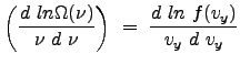 |
|||
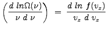 |
Thus, the following equality is clear:
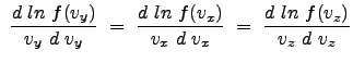 |
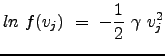
Since the individual functions of x, y, and z are equal to one another for all space, we can justifiably argue that each is a constant (equal in all cases); in general we can write:
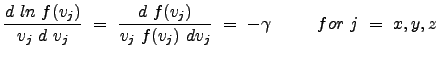 |
We use the negative of a positive ![]() in order to obtain a probability function that is well-behaved as
in order to obtain a probability function that is well-behaved as ![]() approaches
approaches ![]() . The solutions for the previous equation are:
. The solutions for the previous equation are:
 |
|||
 |
|||
This last equation is the general expression of our solution; it applies to the individual probability distributions in each direction (x,y,z) (recall we decomposed our total distribution into a product of the three individual distributions).
We still need to consider 2 missing elements:
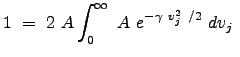
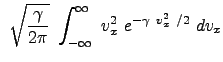
To determine an expression for ![]() , we need to consider that the distribution is normalized over the domain for which it is defined. What does this mean operationally? Since this expression represents a probability, the sum of the individual probabilities for each infinitesimal region of space (or in this case, each window in `velocity" space) must sum to 1. Thus we have:
, we need to consider that the distribution is normalized over the domain for which it is defined. What does this mean operationally? Since this expression represents a probability, the sum of the individual probabilities for each infinitesimal region of space (or in this case, each window in `velocity" space) must sum to 1. Thus we have:
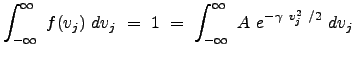 |
|||
 |
|||
 |
|||
 |
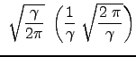
We used the property of even integrands to change the lower limit of integration. Thus, the distribution becomes:
 |
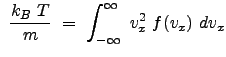
To evaluate ![]() , we introduce from statistical mechanics (which we just state here without proof, which is left for another course or to the
individual student):
, we introduce from statistical mechanics (which we just state here without proof, which is left for another course or to the
individual student):
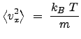 |
where ![]() is the mass of the particles. Thus,
is the mass of the particles. Thus,
 |
|||
 |
|||
 |
|||
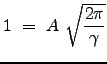
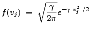
We have thus arrived at the famous Maxwell-Boltzmann velocity distribution in one dimension:
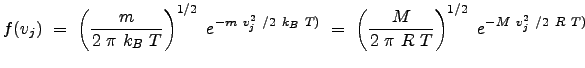 |
where mass, ![]() , is in units of
, is in units of ![]() and molar mass,
and molar mass, ![]() , is in units of
, is in units of
![]() (we use the relation
(we use the relation
![]() for the conversion between the forms using
for the conversion between the forms using ![]() and
and ![]() .
.
In three dimensions (Cartesian represenatation) the total distribution becomes:
 |
|||
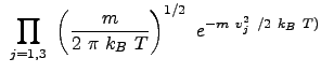 |
|||
|
Example Problem 33.1 (Engel and Reid)
 |
|||
 |
|||
 |
|||
The result reflects the vectorial nature of velocity.