This week, we will first continue what we started in lab07, by doing some more practice with creating M-files that define new MATLAB functions, and with scripts that test those M-files.
We will then use these new functions to develop our lab06 software a bit further by
Other references for the "design recipe" idea:
Also see Chapter 5 in your textbook for information on M-files that define a function.
Before starting this lab:
axis function described on p. 117 (Chapter 3).Create a new subdirectory ~/cisc106/lab08, and make that your working directory.
If you are not sure how to do this, then review the instructions from lab03, steps 1a through 1d.
There are two ways to copy the files for this week's lab. Read over both methods before deciding which one to use.
/www/htdocs/CIS/106/pconrad/06F/labs/lab08
Assuming that you are already in ~/cisc106/lab08 as your current working directory, the following command will copy all the files you need.
cp, and right after the *>> !cp /www/htdocs/CIS/106/pconrad/06F/labs/lab08/* .
>>
There are additional notes about this command at lab04, step 1b if you need to review how this command works.
The work you do in step 2 of this lab is only for practice and learning. There is nothing to turn in from this step of the lab. But it is still important and required.
In lecture on October 13, we developed a file called sumUpToK.m. That file is making a reappearance, but now in the context of the "design recipe" idea, along with a script file for doing regression testing on it.
Look at the files sumUpToK.m and testSumUpToK.m. Look at these files and try to understand how they work. Try running testSumUpToK.m. Also try a few of the examples at the command line, to see what the output is, e.g.:
>> testSumUpToK
...


>> sumUpToK([4 2 9 1 3],3)
...

>> sumUpToK([4 2 9 1 3],4)
...

>> sumUpToK([4 2 9 1 3],0)
...

>> sumUpToK([4 2 9 1 3],5)
...

>> sumUpToK([4 2 9 1 3],6)
...
Look inside these two M-files and understand how they work. It is crucial that you understand this before continuing. Ask your TA for help if you don't understand, and/or, come to see the instructor during office hours.
Look next at isLeapYear.m and testIsLeapYear.m. Try to understand how they work. Try a few examples at the command line, and see what output you get.
>> testIsLeapYear
...


>> isLeapYear(2004)
...

>> isLeapYear(1997)
...

>> isLeapYear(2000)
...

>> isLeapYear(1900)
...
Look at the M files also. Note the nested if/else inside of isLeapYear.m. You need to be able to read and understand this code and how it works before going on, because later steps depend on that understanding.
Also, be sure you understand the idea of regression testing (as introduced in Step 2b of lab07)—the idea of writing a separate M-file that defines a script (e.g. testIsLeapYear.m) to test an M-file that defines a new MATLAB user-defined function (e.g. isLeapYear.m). Go back and review Step 2b of lab07 if you are not clear on this point.
Take a look at cisc106URL.m. This file defines a very useful user-defined function. It is based on the idea of refactoring—that is, taking part of your existing code, and factoring it out into a separate file.
The code inside cisc106URL.m is part of the hurricane.m script that we used in lab06. However, we have parameterized it by specifying a function that consumes a lab number (as a string, e.g. 'lab06' or 'lab08'), along with a jpeg filename, and produces the URL that would be used to retrieve that from the web.
Try running this file on a few examples, as shown below. Note that your output will be different from mine, because it will reflect your userid.
You'll also note the URLs returned are not the ones of any files that actually exist—they are just the addresses of where we would normally place the files on the web if we used our standard naming conventions:
>> cisc106URL('lab08','foo.jpg')

ans =

http://copland.udel.edu/~pconrad/cisc106/lab08/foo.jpg

>> cisc106URL('lab06','foo.jpg')

ans =

http://copland.udel.edu/~pconrad/cisc106/lab06/foo.jpg

>> cisc106URL('lab06','plotWind.jpg')

ans =

http://copland.udel.edu/~pconrad/cisc106/lab06/plotWind.jpg

>> cisc106URL('lab08','plotTemp.jpg')

ans =

http://copland.udel.edu/~pconrad/cisc106/lab08/plotTemp.jpg

>>
Look inside this file and understand how it works.
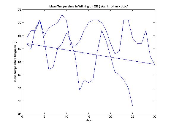
Often you can learn a great deal from looking at a failed attempt at doing something. The testPlot1.m file is an example of this.
First, let's point out that testPlot1.m is not a complete failure. It does illustrate one thing very well:
But, it doesn't do its main job very well, which is to produce a plot of the mean temperature in Wilmington Delaware (from the file sepOctTemps.dat). Try running it, and look at the graph that is produced. It will probably look something like this:
The problem is that we are plotting the "day" field on the x-axis, and the day field "starts over again" at 1 when we move from September into October. So the plot is messed up... the line returns to the left of the graph, and starts over again, plotting from left to right.
Instead, consider the file tempPlot2.m.
Note: You won't be able to run this file, because I have NOT provided you with a complete working version of the function ordinalDay.m, which is needed!
But you can look at how it works, and see an example of the plot it produces (shown below):
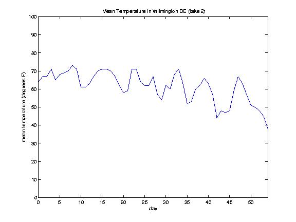
Notice a few things:
axis function to make the plot look neater. This allows us to define the extent of the x and y axis. This is how we can avoid the problems we saw in lab06 of the wind plot being "coincident" with the edges of the graph. ordinalDay to compute the day of the year, and then subtracting to get elapsedDays, and plotting elapsedDays, instead of plotting day. This makes the graph turn out properly.
Clearly, this file is meant to illustrate several improvements that you can make to your lab06 file. That's what the rest of this lab is about. But first, we have to write and test the function ordinalDay.m
I've provided you with a "stub" for ordinalDay.m. This is a file that has the first two steps of the design recipe worked out.
I've also provided you with testOrdinalDay.m, which can be used to complete step 4 of the design recipe.
If you run testOrdinalDay.m now, it will show that all six tests fail.
>> testOrdinalDay

  Results for ordinalDay:

  0 tests passed, 6 tests failed

>>
Your job is to carry out step 3, and fix the body of ordinalDay.m so that all six tests pass.
Write the body of the function, and test it. When all the tests pass, you know you are done!
The idea of the ordinalDay function is this: given a month, day and year, determine what day of the year that is (the so-called ordinalDay). For example:
You can test this function in three ways:
When your function is complete and it tests ok, continue to the next step:
You can use either a unix command to copy from lab06/lab06.m file to your lab08/lab08.m (you need to be in your cisc106 directory to do that), or you can use MATLAB's file browser, and do a "Save As".
Change the references inside the file from lab06 to lab08. Make sure it still works.
Then take out all the detailed steps needed to produce the plot, and replace those with a simple call to the cisc106plot() function. When you do this, be sure that the filename you pass into the cisc106plot() function has the .jpg extension. The MATLAB strrep() function may be useful as you go about this.
Compute the min and max of the wind vector, and set the edges of the graph to be 10 mph lower then the min and 10 mph higher than the max, using the MATLAB axis function, as illustrated above in step 2.
The idea here is to construct an elapsed time vector that reflects the number of hours that have elapsed from the first line of the file. You can do this by first computing two intermediate results:
You can then multiply elapsed days by 24, and add it to elapsed time (which in the case of a negative value, is actually a subtraction), to compute the elapsed time.
Your diary file should contain the following:
Be sure that the URLs that appear when you run your lab08.m file link to files on the web that are readable, and that contain valid graphs of the results from that particular hurricane. Also be sure that the edges of the plot don't touch the top or bottom of the graph. This should be because of the code you added in step 4c, not because of a "careful choice of data files". :-)
Upload and submit the following files:
That's it for lab08!
Due 11:55pm Thursday November 16, with NO LATE PENALTY for submissions by 11:55pm Friday November 17.
Penalties for late submissions:
ordinalDay.m function: 20 pointstestOrdinalDay.m script: 10 points lab08.m script: 40 points, broken down as follows