This week, in lab03, you will learn how to start with a simple data file of numbers—in this case, data about Hurricane Katrina (from August of 2005)—and end up with two graphs
In the process, you'll also learn a few things about slicing up Matrices in MATLAB, i.e. selecting out particular rows and columns.
Next week, in lab04, we'll add two more graphs:
And we'll also learn a little bit of HTML so that we can incorporate all four graphs into a simple web page.
By the time you complete this lab, you should be able to:
You will also get more practice with
pwd, mkdir, and cd commands.Reasons (and the possible ways around them)
You can review the instructions from lab01 for starting up MATLAB on the SunRays if you are not sure how to do this.
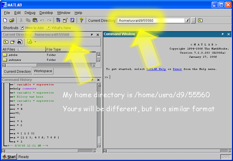
When you first startup Matlab, you will likely start out in your "home directory", just like last week, as indicated in the diagram below. (again, mine is /home/usra/d9/55560—yours will be different from that, but still in a similar format:).
You can do this in one of two ways.
cd cisc106 in the command window cisc106 folder in the current directory window.
Now, in the MATLAB command window, type pwd, like this. The answer that comes back should show you your cisc106 directory under your home directory, like this:
>> pwd

ans =

/home/usra/d9/55560/cisc106

>>
That tells you that you are in the right place.
To do this, type the following three commands in the MATLAB command window. Note the use of lowercase—in general don't use capital letters in MATLAB except when the instructions specifically indicate to do so! (An explanation of each command follows the example input/output)
>> mkdir lab03
>> cd lab03
>> pwd

ans =
    /home/usra/d9/55560/cisc106/lab03
>>
mkdir lab03 , makes a new subdirectory (folder) called lab03. This is the folder where you will store all of your work for lab03 cd lab03 , changes your current directory to be this new lab03 directory.pwd, asks MATLAB to print the working directory. Note that the working directory is now your home directory with cisc106/lab03 stuck on the end of it.This is probably the last week that all of this will be spelled out in so much detail. In future weeks, I'll just give you a very general instruction such as the following one. Note that the tilde (squiggle) symbol (~) stands for "your home directory":
lab04 subdirectory under your ~/cisc106 directory, and change your working directory to ~/cisc106/lab04.You'd be expected to either (a) remember how to do that, or (b) look back at lab02 or lab03, and figure it out.
A few things to remember (this is review from lab02):
cd .. (that's cd dot dot).cd ~ (that's cd squiggle) At the following web link, there is a file called katrina.dat. This file contains some data about Hurricane Katrina, which affected the Gulf Coast of the United States in August 2005, particularly in the city of New Orleans and areas of nearby states.
This file is also available on strauss (and from within MATLAB on the SunRays) in the directory:
/www/htdocs/CIS/106/pconrad/06F/labs/lab03/katrina.dat
A description of this data file is at this link:
The contents of that files are repeated here for your convenience:
Data in katrina.dat is summarized  from
the web page http://www.wunderground.com/hurricane/at200511.asp

The columns represent:

Column 1: Time(GMT)
Column 2: Day of Month (All August 2005)
Column 3: Latitude (N)
Column 4: Longitude (w)
Column 5: winds (mph)
Column 6: pressure (millibars)

For example, the first four rows are:

18  23  23.1   75.1      35    1008
 0  24  23.4   75.7      35    1007

The first row indicates that at 18 hours GMT on August 23 2005,
Katrina was at latitude 23.1 north, and 75.1 west.  Maximum winds
winds were 35 mph, and the pressure was 1008 millibars.

18 hours GMT corresponds to 13 hours Central Daylight Time, i.e. 1pm.
(CDT is the time zone for New Orleans).  CDT is GMT minus 5.
My source for that information
is the web page: http://www.dxing.com/utcgmt.htm

The second row indicates that at 0 hours GMT on August 24 2005,
(i.e. midnight, or 24-5 = 19 hours CDT, or 7pm on August 23)
Katrina was at latitude 23.4 north, and 75.7 west.  Maximum winds
winds were 35 mph, and the pressure was 1007 millibars.
To copy this file into your ~/cisc106/lab03 directory, you can type the following command in the MATLAB command window. Note a few important details:
cp command is a Unix command to "copy a file". cp the part that is /www/htdocs/CIS/106/pconrad/06F/labs/lab03/katrina.dat is the file you are copying "from". .) This dot is a symbol for "the current directory", which is the place you are copying "to". >>!cp /www/htdocs/CIS/106/pconrad/06F/labs/lab03/katrina.dat . >>
To see if it worked, you can do one of two things—actually, if possible, you should do both:
dir in the command window. This means "list the files in my directory".
. and .. in that folder are symbols for the current directory, and the parent directory (which should be cisc106)>> dir
. .. katrina.dat >>
If you are working on your PC, then create a directory cisc106 somewhere, and a directory lab03 under it. Then use your web browser to find the katrina.dat file and save it into that directory.
katrina.dat into a MATLAB matrix called katrina The file katrina.dat is an example of an "ASCII formatted data file." You can read more about these in Section 2.7 of your text (pages 43 through 45), which I recommend you read over before you continue.
We are going to use the command load katrina.dat to load the contents of that file into a MATLAB matrix called katrina. Try the following commands—hopefully your results are as shown below.
>> load katrina.dat
>> katrina

katrina =

   1.0e+03 *

    0.0180    0.0230    0.0231    0.0751    0.0350    1.0080
         0    0.0240    0.0234    0.0757    0.0350    1.0070
    0.0060    0.0240    0.0238    0.0762    0.0350    1.0070
    0.0120    0.0240    0.0245    0.0765    0.0400    1.0060
    0.0180    0.0240    0.0254    0.0769    0.0450    1.0030
         0    0.0250    0.0260    0.0777    0.0500    1.0000
    0.0060    0.0250    0.0261    0.0784    0.0600    0.9970
    0.0120    0.0250    0.0262    0.0790    0.0650    0.9940
    0.0180    0.0250    0.0262    0.0796    0.0700    0.9880
         0    0.0260    0.0259    0.0803    0.0800    0.9830
    0.0060    0.0260    0.0254    0.0813    0.0750    0.9870
    0.0120    0.0260    0.0251    0.0820    0.0850    0.9790
    0.0180    0.0260    0.0249    0.0826    0.1000    0.9680
         0    0.0270    0.0246    0.0833    0.1050    0.9590
    0.0060    0.0270    0.0244    0.0840    0.1100    0.9500
    0.0120    0.0270    0.0244    0.0847    0.1150    0.9420
    0.0180    0.0270    0.0245    0.0853    0.1150    0.9480
         0    0.0280    0.0248    0.0859    0.1150    0.9410
    0.0060    0.0280    0.0252    0.0867    0.1450    0.9300
    0.0120    0.0280    0.0257    0.0877    0.1650    0.9090
    0.0180    0.0280    0.0263    0.0886    0.1750    0.9020
         0    0.0290    0.0272    0.0892    0.1600    0.9050
    0.0060    0.0290    0.0282    0.0896    0.1450    0.9130
    0.0120    0.0290    0.0295    0.0896    0.1250    0.9230
    0.0180    0.0290    0.0311    0.0896    0.0900    0.9480
         0    0.0300    0.0326    0.0891    0.0600    0.9610
    0.0060    0.0300    0.0341    0.0886    0.0450    0.9780
    0.0120    0.0300    0.0356    0.0880    0.0350    0.9850
    0.0180    0.0300    0.0370    0.0870    0.0350    0.9900
         0    0.0310    0.0386    0.0853    0.0350    0.9940
    0.0060    0.0310    0.0401    0.0829    0.0300    0.9960

>>
Compare the first three lines of output in the window above, namely:
>> load katrina.dat
>> katrina

katrina =

   1.0e+03 *

    0.0180    0.0230    0.0231    0.0751    0.0350    1.0080
         0    0.0240    0.0234    0.0757    0.0350    1.0070
    0.0060    0.0240    0.0238    0.0762    0.0350    1.0070
...
with the actual contents of the first three lines of katrina.dat, which are:
18  23  23.1   75.1      35    1008
 0  24  23.4   75.7      35    1007
 6  24  23.8   76.2      35    1007

...
MATLAB has the correct matrix, but it is in a rather odd format—specfically, all the values have to be scaled by 1.0e+03 (i.e. 1.0x10³) to get the true value. That's the meaning of the the first part of the MATLAB output for the matrix called katrina, namely the 1.0e+03 * on the first line of the output for the matrix katrina.
We can tell MATLAB to give us the numbers in a nicer format with the command format short g, as shown below. Read about the format short g command (and other related commands) on pages 40 and 41 of your text (section 2.6), and try the command out below. You might also try some of the other commands on p. 41, to see what the matrix looks like with those formats.
>> format short g
>> katrina

katrina =

           18           23         23.1         75.1           35         1008
            0           24         23.4         75.7           35         1007
            6           24         23.8         76.2           35         1007
etc... some lines omitted here
            6           31         40.1         82.9           30          996

>>
katrina as a map of longitude and latitudeNow that we have the data into MATLAB, we can do some interesting plots.
The first plot we might do is to plot the coordinates of the latitude and longitude. This should gives us a kind of "map" of where the hurricane went. We'll put longitude values on the x-axis, and latitude values on the y-axis.
This means that we need some way to "select out" the column in our matrix that has the longitude, which is the x-axis. Longitude is the fourth column in the matrix, which we can select out with the command:
longitude = katrina(:,4)
Try that command, without putting the semicolon on the end. (Or you can put the semicolon on, and then type longitude to see what the contents of longitude are.)
The expression katrina(:,4) means the following:
: before the comma means "all rows of katrina" 4 after the comma means "only column 4".Therefore, what we get is a column vector consisting of all the longitude values.
Next, write a command to select out only the third column as the latitude. (I've left this as a "fill in the blank" so you can figure out that command on your own.)
latitude = _____________
And then, finally we can plot:
plot(longitude, latitude);
When we first do this, we get a plot that looks like the following:
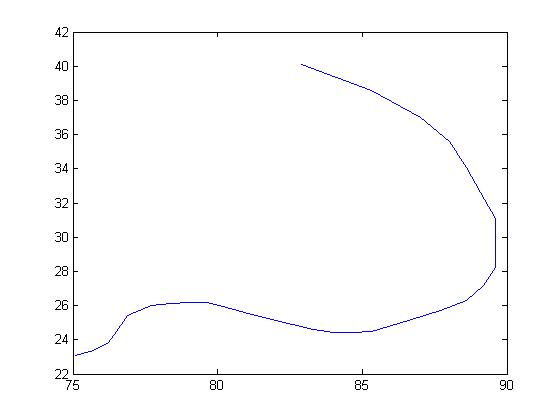
Compare this with the picture at the web link http://www.wunderground.com/hurricane/at200511.asp. You'll notice that the shape of the hurricane's is "backwards" from what it should be. The reason is that the longitude values are values "west of Greenwich", i.e. they should be plotted as negative numbers.
We can fix this by replacing our plot command with the following:
plot(-longitude,latitude);
Note how this corrects the shape of the plot.
lab03a.m Now we are ready to make an M-File to do all this. Below, I've given you most of what you need for this M-file, to help get you started. We are also going to add two more commands as we turn this into an M-file—here's an explanation of those:
legend command puts a legend on the graph. You can read more about this in Section 2.11 of your text, particularly on p. 60.
"), but two single quotes ('')—so that MATLAB knows that the message isn't over yet.
legend('Katrina''s path');title command puts a title at the top of the graph.
title('Donald Duck''s map of Hurricane Katrina''s path'); Call your M-file lab03a.m, and put the following commands into it, EXCEPT:
Donald Duck to your name in both places where it appears 019 to your section number09/13/2006 to the actual date you finish the lab latitude
% lab03a.m
% Donald Duck, section 019 for CISC106 lab03, 09/13/2006
% Plot a map of the path of hurricane Katrina

load katrina.dat;
longitude = katrina(:,4);
latitude = ____________;
plot (-longitude,latitude);
legend('Katrina''s path');
title('Donald Duck''s plot of Katrina''s path for CISC106');
After you've typed in this and saved it, run it once to produce the graph. Remember that we run an M-file by typing its name without the .m part (see lab01 and lab02 if you need a refresher on this.)
This week, you don't have to make a diary—instead, your plot will be the evidence that your M-file works. So, we need to save the plot, which is our next step.
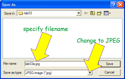
Now, go into the window where the plot is, and go to the menu option File... Save As...
In the window that comes up, at the bottom where it says "Save as type", you need to change this to JPEG, as shown here, and specify lab03a.jpg as your filename:
Once you've done that, you should be able to use the "File... Open File" dialog of your web browser to open the lab03a.jpg file and see your plot as a web graphic (i.e. .JPEG file.) It should open up and display something like this:
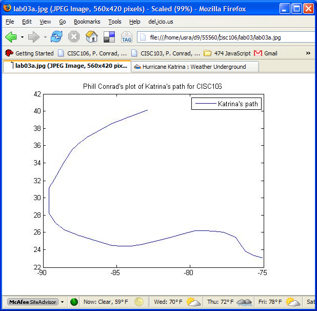
This shows that the graphic can be viewed in a web browser, though we haven't yet shown how to actually put it on the web—that part will come next week.
If you've gotten this far, you are about half way done with this week's lab: you have two of the files you are going to submit.
In all, you are going to submit four files to WebCT: two M-files, and two jpeg files. Here is an overview:
| Step | Plot | M-file name | JPEG file name | |
|---|---|---|---|---|
| x axis | y-axis | |||
| 3 | -longitude | latitude | lab03a.m |
lab03a.jpg |
| 4 | wind speed (mph) | pressure (millibars) | lab03b.m |
lab03b.jpg |
For the last step, I'm giving you only an oveview of what to do. The detailed steps are up to you to figure out.
Fortunately, they are very similar to what you already did in Step 3, so you should be able to figure it out without too much trouble.
What to do:
When you've produce those two files, you are ready to submit.
You should upload and submit your two M-files, and your two JPEG files on WebCT—then, you are done!