
The single most time-consuming operation in statistical analysis is preparing the data for use in the statistical procedures. Data preparation consists of several operations, including --
Remember, very little happens in the SAS system until data are put into a SAS data set. A SAS data set is stored in a "binary" format and looks like garbage when viewed in a text editor or unix pager like less. For example, the gss04 data set looks like --
SAS can read it, but people can't. However, you can display it with Viewtable.
Any data not stored in a SAS data set must be copied into a SAS data set before much can be done with it. The source data are not changed by this operation. For example --
  data income;
    infile "~larryh/lab2/income1000.data";
    input  Black     1
           othrace   2
           female    3
           Age       4-5
           Educ      6-7
           edlths    8
           Edjc      9
           edcoll    10
           edgrad    11
           Hours     12-13
           weekswrk  14-15
           partfull  16
           prestg80  17-18
           annInc    19-26;
    ageSq=(age-46)**2;
    logAnnInc=log(annInc);
  run;
does not change the input text file, ~larryh/lab2/income1000.data. It just copies it, creates two new variables and saves the combined result in a temporary SAS data set named income.
Probably ASCII text files are the most frequently encountered format of non-SAS data, often called external data sources. ASCII text files are files you can read with a text editor or pager. The first few lines of ~larryh/lab2/income1000.data", for example, are --
001381200004052128 27.7160
001441300002552122 31.8296
001241200002830138 10.6590
001451600104430151 14.8407
000401200004848134 19.2620
001541200005252147 12.3058
000241401004052174 34.7468
00044 510004052122 35.8491
001621300008948130 11.8894
001361400006552132 66.8078
But external data are stored in many formats other than ASCII (MS Excel, MS Access, SPSS, Stata, SAS transport). Probably the most common format for data collected by individuals (contrasted to institutions) is Excel. The next few examples come from the SAS sample files located in --
/opt/sas9.1.3/dist/samples/stat/regex.sas
An excerpt from this file is --
  data Class;
    input Name $ Height Weight Age @@;
    datalines;
Alfred  69.0 112.5 14  Alice  56.5  84.0 13  Barbara 65.3  98.0 13
Carol   62.8 102.5 14  Henry  63.5 102.5 14  James   57.3  83.0 12
Jane    59.8  84.5 12  Janet  62.5 112.5 15  Jeffrey 62.5  84.0 13
John    59.0  99.5 12  Joyce  51.3  50.5 11  Judy    64.3  90.0 14
Louise  56.3  77.0 12  Mary   66.5 112.0 15  Philip  72.0 150.0 16
Robert  64.8 128.0 12  Ronald 67.0 133.0 15  Thomas  57.5  85.0 11
William 66.5 112.0 15
     ;
  run;
The data in this example are displayed in three blocks of columns. There are only four variables (Name, Height Weight, Age), but 12 data fields in the data following the datalines statement. The trailing double at sign (@@) indicates to hold each line until all its contents are read. Also note the dollar sign ($) following the Name variable. It signifies a text string or character variable. This formating of text data probably is unusual in general, but it's often used in SAS documentation.
A more-frequently used format is the one we've seen before: Each line of data represents one observation. The same data rearranged to this format looks like --
Name    Height  Weight  Age
Alfred  69      112.5   14
Carol   62.8    102.5   14
Jane    59.8    84.5    12
John    59      99.5    12
Louise  56.3    77      12
Robert  64.8    128     12
Alice   56.5    84      13
Henry   63.5    102.5   14
Janet   62.5    112.5   15
Joyce   51.3    50.5    11
Mary    66.5    112     15
Ronald  67      133     15
Barbara 65.3    98      13
James   57.3    83      12
Jeffrey 62.5    84      13
Judy    64.3    90      14
Philip  72      150     16
Thomas  57.5    85      11
William 66.5    112     15
which, assuming this data file is named HtWtAgeData.dat, can be read with --
  data class;
    infile "HtWtAgeData.dat" firstobs=2;
    input Name $ Height Weight Age;
  run;
Compared to the previous command file, note the absence of the double trailing at signs and the presence of the option on the infile statement: firstobs=2.
An Excel file with one worksheet arranged to appear like this --
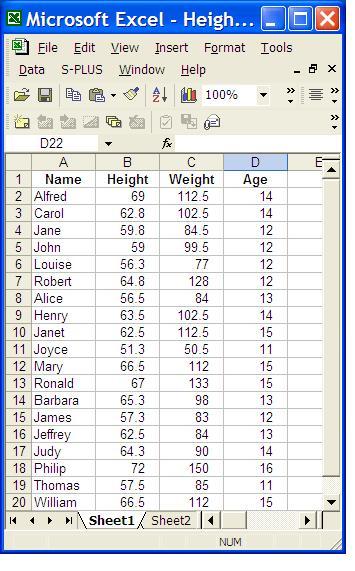
can be read by UNIX SAS --.
  options ls=80 noovp;

  proc import
       dbms=xls datafile="HeightWeightAgeData2.xls"
       out=class;
  run;
(Assuming the Excel file is named HeightWeightAgeData2.xls).
Windows SAS also can read an MS Access table --
  options ls=80 noovp formchar='|-    +';

  proc import table="HtWtAge" out=AgeWtHt dbms=access97;
    database="HeightWeightAge.mdb";
  run;

  proc print;
    id name;
    format name $char10. Height Weight 5.1 Age 2.0;
  run;
but UNIX SAS cannot.
UNIX SAS also can read and write SPSS (.sav) system files and Stata system files (.dta).
To read an SPSS system file, upload it from Windows using Secure Shell (SSH). Then syntax like --
 * BreastCancerSurvival.sas: Read the SPSS system file
            containing breast-cancer survival data. *;

  options ls=80 noovp formchar='|-    +';

  proc import out=BCSurvival
       datafile='Breast cancer survival.sav';
  run;
  proc datasets lib=work nolist;
    modify BCSurvival;
    format ID z4.0 age lnPos 2.0 histgrad 2.0
           pathsize 6.2 time 4.2;
  run;

  proc contents data=BCSurvival; run;

  proc print data=BCSurvival(obs=20); id ID; run;
can be used to import it.
The current version of Stata (V9) does run on strauss. So you can read a Stata system file without necessarily uploading it from a Windows machine. For example --
 * autoData.sas: Read the Stata system file containing the old
                 automobile data. *;

  options ls=80 noovp;

  proc import out=autoData
              datafile='/opt/stata9/auto.dta'; run;

  proc datasets lib=work nolist;
    modify autoData;
    format rep78 2.0
           headroom 3.1
           trunk 4.2
           weight 4.0
           length 3.0
           turn 2.0
           displacement 3.0
           gear_ratio 6.3
           price 5.0
           foreigh 2.0;
  run;

  proc contents data=autoData; run;
  proc print data=autoData(obs=20); id make; run;

  options nolabel;
  proc means maxdec=3 data=autoData; run;

  proc freq data=autoData;
    tables foreign make turn;
    tables  make*foreign / nopercent norow nocol;
  run;

  proc logistic data=autoData descending;
    model rep78 = foreign displacement weight;
  run;

  proc reg data=autoData;
    model mpg = weight displacement gear_ratio
                foreign;
  run;
reads one of the sample data sets that comes with Stata, sets variable formats using the datasets procedure, prints the contents of the data set, and runs some statistical procedures.
Some major data sources such as the Medical Expenditures Panel Survey (MEPS) can be downloaded in SAS transport format. This is a handy way to get the data if you plan to use SAS to analyze it and/or do your data preparation. The copy procedure can be used to import the MEPS SAS transport files. For example --
 * h89.sas: Read meps h89 SAS portable file *;

  libname meps2004 xport "H89.SSP";

  proc copy in=meps2004 out=work; run;

  data h89;
    set h89;
    if 0 < ADGENH42 <= 5 then ADGENH42 = 6-ADGENH42;
    else ADGENH42=.;
    if age04x < 0 then age04x = .;
    if VETVIET < 0 then VETVIET = .;
    female=sex-1;
    male=2-sex;
  run;

  proc contents; run;

  proc freq data=h89;
    tables sex age04x actdty53 ADGENH42 VETVIET;
    tables VETVIET*sex / norow nopercent;
  run;

  proc logistic data=h89 descending;
    model ADGENH42 = female age04x female*age04x
          VETVIET male*VETVIET;
  run;
reads the 2004 MEPS data, prints the contents of the data, does some elementary data prepration and runs some statistical procedures.
In general, when analyzing medium to large amounts of data, it's advisable to organize your work into at least two parts:
One of several advantages to this split is that it speeds up your analysis. With the MEPS data and in the previous example, compare the combined rudimentary data preparation and analysis combined in one SAS session --
to --
and --
The combined run (h89.sas) takes a total of about 1 minute, 8 seconds to run. The data-preparation part of this consumes nearly one full minute (h89Dataprep.sas) -- 57.57 seconds. But the statistical analysis part (h89Stats.sas) takes just 20.97 seconds. (No, they don't add up!) In this case, you save about 40 seconds of "real time" each time you do an analysis run because you don't import the data and do the calculations in the data step before you get to the stats. Also, there is no point in running the contents procedure and descriptive stats every time (but you may want them on file from the initial run).
But saving run time is not the only advantage of organizing your work int dataprep and analyses phases. Typically, beginners build up an input program in small increments, tacking the analyses they want on the bottom of the program, after the data step. Soon the amount of output generated by adding more and more statistical analyses at the bottom of the input program becomes unmanageable. Two strategies typically are used to avoid excessive output --
With the first strategy, the length of the program rapidly grows to several screens. It becomes increasingly difficult to debug, partly because it often is not obvious whether the code you are looking at is part of a comment.
With the second strategy, when the inevitable errors are discovered in
the input program, or new variables are needed, then changes must be
made in many places instead of just one. Often several
different copies of the input program exist and it is difficult
to tell which is correct and which contains which
variables.
A second important reason to separate the data preparation and analysis, then, is to reduce the size of your programs and help manage the complexity of a large project.
In summary: Creating permanent SAS data sets is an important conceptual step. The primary advantages of doing so are --
The primary disadvantage of creating a permanent SAS data set is: it consumes disk storage space. You can request an increase in your quota online. Go to the Network page off the home page for the University of Delaware, login using your UD netID and password and select ° Request a disk quota change. Note that you can get up to 5GB on the scratch disk with no questions asked. Files stored on scratch are permanent files, but they are not backed up (in contrast to files stored elsewhere).
Data from some source must be used as input to the working SAS data set. Usually the source data are stored in a non-SAS format, but not always. Possible formats of source data include (but are not limited to) --
  data income;
    infile "~larryh/lab2/income1000.data"
    input  Black     1
           othrace   2
            .
            .
            .  ;
  proc import dbms=xls datafile="HeightWeightAgeData2.xls"
                       out=class;
  run;
  proc import table="HtWtAge" out=AgeWtHt dbms=access97;
    database="HeightWeightAge.mdb";
  run;
  proc import out=BCSurvival
              datafile='Breast cancer survival.sav';
  run;
Stata example --
  proc import out=autoData
              datafile='/opt/stata9/auto.dta';
  run;
  libname meps2004 xport "H89.SSP";
  proc copy in=meps2004 out=work; run;
Note the unusual form of the libname statement. It contains the xport option, and the quoted string is a filename not a directory.
  libname wrds " ... ";
  libname thesis  ".";

  data thesis.crspdata;
    set wrds.crsp;
Permanent SAS data sets are identified by a two-part name, OR by a quoted string.
Two-part name: The form of the first method is --
<libref.dsname>
A period separates the parts. In contrast, temporary SAS data sets generally are identified by a one-part name, as we have seen in previous exercises.
The libref identifies a UNIX directory; the libref name is established by the libname statement in SAS. For example, the following libname statement --
libname lhsas '~larryh/sasnotes';
gives the name of lhsas to the libref and associates it with the UNIX directory called ~larryh/sasnotes.
Another way to think about this abstraction is that the libname statement defines an alias or synonym for a UNIX directory, in this example ~larryh/sasclass, to be used in the rest of the job. SAS calls this alias a "libref." It must conform to all the conventions for SAS names: start with a letter or underscore and contain only letters, underscores, or numbers. But, unlike most SAS names, its length may not exceed eight (8) characters.
The dsname is the name of the data set. It also must conform to the conventions of SAS names, and can be up to 32 characters long. The connection between the dsname and the UNIX filename is: The dsname is the root part of the UNIX filename. The extension is defined by SAS. It is sas7bdat.
Quoted string: One also can identify a permanent SAS data set by enclosing its UNIX file name in quotes. But this is not quite as simple as it might seem at first. The file extension must be sas7bdat, like this --
"<dsname>.sas7bdat"
For example, using the two-part name method, you can save a permanent sas data set in your sasclass directory with the statements --
  libname sasclass '~/sasclass';
  data sasclass.gss04;
    .
    .  <code to input data>
    .
  run;
This produces a UNIX file named gss04.sas7bdat in your sasclass directory. SAS automatically adds the .sas7bdat extension. This is how SAS recognizes SAS data sets.
Exactly the same result is produced using the quoted-string method of identifying the SAS data set --
  data 'gss04.sas7bdat';
    .
    .  <code to input data>
    .
  run;
Here you don't need the libname statement. But your current working directory must be sasclass to assure the file is saved in that directory. OR you can enclose the directory name in the quoted string ("~/sasclass/gss04.sas7bdat")
The next exercise illustrates saving a permanent SAS data set and a recoding operation on income. It also includes computation of descriptive statistics, frequencies and histograms.
The values of income as read in from the GSS are codes representing income intervals. The distances between the boundaries of these intervals differ quite substantially from one interval to the next. Hence, serious analysis of income may benefit by recoding to the midpoint of the income intervals.
It often is convenient to code annual income into thousands of dollars. For example, the GSS code for rincom98 of 17 stands for the income interval of 35,000 dollars to and including 39,999. We might therefore recode 17 to the midpoint of this interval in thousands of dollars (35+40)/2=37.5. Some arbitrary number must be picked for the upper income category, since it is open ended. (Or, an estimate can be calculated by assuming an income distribution such as Pareto or log-normal). The lowest category may appear open ended, but, in fact, it is bounded at zero.
Copy gssread.sas back into the Program Editor. First, make changes needed to save the SAS data set as a permanent file. Use the two-part name method: Insert a libname statement before the data statement, and edit the data set name on the data statment.
Then add the first three income-recode statements: Place the cursor in the prefix area beside
if rincom98 > 23 then rincom98=. ;
Insert 5 lines by typing i5
 in the prefix area. Then type in the first few
commands to create a recoded income variable, like this --
in the prefix area. Then type in the first few
commands to create a recoded income variable, like this --
To reduce the amount of typing, copy the rest of the income recodes and some procedure commands from a file. But first delete all the lines below the last else if statement you just typed. Then put the cursor on the next line and copy the rest of the program from a file named bottomGssread.sas in my sasclass directory. Select File/Open then type --
~larryh/sasnotes/bottomGssread.sas
into the dialog box at the top of the window. Note that *.sas already is entered in the box.
Now, run the job and view the results.
There are several important observations --
By default, proc chart assumes variables are continuous and tries to collapse their values into intervals for plotting. This is the reason for indicating the discrete option for race and sex. But, if persinc were charted with the discrete option, the skew now apparent in income would not show up on the chart.
Before continuing, go to your UNIX terminal and remove the sas data set you just created (to save your disk quota). Then check your quota with the quota command and the -v flag --
  rm gss04.sas7bdat
  quota -v
A handy device is to store frequently-used SAS statements in a file named autoexec.sas. For example, if the following statements are stored in autoexec.sas --
  options ls=80 noovp;

  libname lhsas "~larryh/sasnotes";
  libname library "~larryh/sasnotes";
you do not need to type them in every SAS session. They are included automatically. The autoexec.sas file may be stored in your home directory or any subdirectory. When it is stored in your home directory, it is executed for all SAS sessions. When it is stored in a subdirectory, it is executed only when SAs is started in the subdirectory where it exists.
Many of the analyses in the next section make use of variables not now in the permanent SAS data set you just created. Instead, we will use lhsas.gss04 data on my account. It contains all the features we will need.
This example of a data step --
The program is stored in a file called dataprep.sas, located in one of my directories.
Note --
