DEPARTMENT OF POLITICAL SCIENCE

AND

INTERNATIONAL RELATIONS

Posc/Uapp 815

Descriptive Statistics

(Continued)

CLASS 7 AGENDA:

Interpretation of hinges
The arithmetic mean
The standard deviation and variance, measures of dispersion

Summation notation

Reading:

Agresti and Finlay, Statistical Methods, pages 45 to 67. (Look for the topics we're covering.)

INTERPRETATION OF DISPLAYS AND ORDER STATISTICS:

The stem-and-leaf display is analogous to frequency distributions and histograms described in most basic statistics texts, but is easier to calculate and draw. It also simplifies the computation of other exploratory statistics.
The interpretation of the hinge:

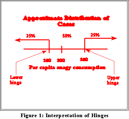
See Figure 1. 50 percent of the cases (states) lie between 280 BTUs per capita and 380 BTUs. Note that the hinges scores are not equally distant from the median.

What interpretation can we put on these numbers? The median is fairly self-explanatory in this case. It represents the middle or typical value in that some states have lower, some higher per capita rates of energy consumption.
Now look at the variation. Lets look at the "middle" 50 percent of states, the ones between the hinges, which are 280 and 380. So apparently there is not much variation in energy consumption among the middle group of states. After all, the difference is only 100 BTUs. Moreover, we see from the stem-and-leaf display that most values are within few hundred BTUs of average. Only a few states have relatively high rates of consumption.

An important task might be to identify those places and decide why they are considerably above average.
We can contrast this "amount" of variation with a situations where there is much more or much less, just to see how hinges might be used to assess differences.

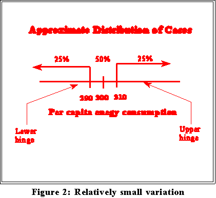
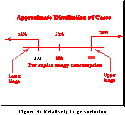
Figure 2 shows limited variation: 50 percent of the states lie between 290 and 310 BTUs. In Figure 3, by contrast there is much more variation because the middle 50 percent of cases extend from 300 to 480.

In moment we will add maximum and minimum values to create a "boxplot" that presents and even clearer view of variation.
A key question is: why is there such great variation? As I mentioned in the previous class, part of the explanation may lie in cross-national differences in attitudes and approaches to illness and health care.

What MINITAB does:

MINITAB stem-and-leaf displays will not look like yours (usually) but the letter values should be the same, except that MINITAB calculates more of them.

THE MEAN:

To repeat what was said in an earlier class, the mean is the sum of all values in the batch or sample divided by the total number, N, of values
Formula for a batch of numbers or sample:

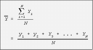
Symbol for the sample or observed mean is , which is read "Y bar." For a population (see later) the mean is denoted with the lower case greek letter mu, .
Summation: The summation symbol, sigma, means addition In particular, it tells you what and how to add.

means add Y₁, Y₂, and so forth until the last data value (the Nth) is reached.
Here is an example. Suppose we have 5 numbers: 10 20 30 40 50.

The summation symbol

means let add the first observation (i = 1), then the second (i = 2), then the third (1 = 3) and so on until i = 5 so stop adding with the fifth number.

This quantity is called the sum of the Ys. In the example, this sum is .

Properties of the mean:

The sum of the deviations from the mean are zero.

In other words, find the mean, , then subtract from each number, and add these "deviations." The total will be 0. Example:

Data: 10 20 30 40 50

= 30

Deviations are (10 - 30) = -20, (20 - 30) = -10...

Sum of deviations is (-20) + (-10) + (0) + (10) + (20)

= 0

In this instance, the sum of squared Ys or sum of squares for short is:

The sum of all squared deviation is a minimum. In other words, suppose we square all of the deviations above (e.g., (-20)², (-10)², etc.) and then add these squares. The sum will be a positive number but it will be at least as small and probably smaller than if we had used some other number besides the mean.

Example:

Data: 5 10 15 70

= 25

Median (M) = 12.5 (why?)

Squared deviations from : Squared deviation from M:

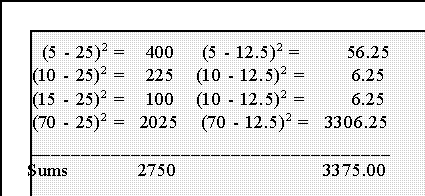
Notice that when deviations are taken from the mean they are smaller than when taken from the median.

As noted in an earlier class, the mean is sensitive to extremely larger or small values. This is a reason why, for example, many studies and government reports use median rather than mean income.

MEASURES OF DISPERSION:

Variation: the total variation in a batch of numbers equals the sum of the squared deviations about the mean.

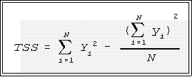
The total variation is also called the total sum of squares.
Its formula is:

In words: for a batch of numbers find the mean, , then subtract it from the first data point and square the difference. Do the same for the second observation, the third and so on. When done add up these squared differences.
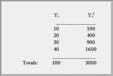
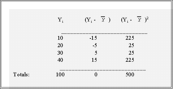
Example: 10 20 30 40

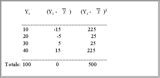
That is,

Computing formula:

When you have lots of data, the total sum of squares can be calculated easily with a good calculator by finding the sum of the Ys' and the sum of the Y's squared; that is:

Then put these quantities in this formula, called a computing formula:

Example:

The total sum of squares is thus:

Variance:

The variance of a batch of numbers or sample is denoted , for a batch of numbers and represents the total variation divided by N minus 1:

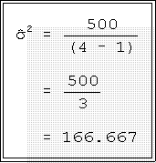
Example: 10 20 30 40

As seen above the TSS is 500. Therefore the variance of this batch of numbers is:

The larger the variance, the more variation or dispersion in the data. But it is difficult to give an intuitive interpretation to any particular value such as 500.

The Standard deviation:

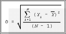
The standard deviation of a batch of numbers or sample, denoted is (loosely speaking) the average of the squared deviations from the mean. Since deviations indicate how much variation exists in the data, having an average of these differences tells one about overall variation.
It is also the square root of the variance.

To calculate the standard deviation, therefore, first obtain the total sum of squares by summing the squared deviations from the mean:

Then divided this total by N - 1, where N is the number of cases in the batch.
Finally, take the square root:

Example: 10 20 30 40; mean = 25

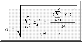
Computing formula:

As be expected, since it is just the square of the total sum of squares divided by N minus 1, the standard deviation can be calculated easily with a good calculator by finding the sum of the Ys' and the sum of the Y's squared; that is (as before):

Put these quantities in the computing formula:

In the previous example, the sum of the Y's squared was 3000 and the sum of the Y's alone was 100 so:

A simpler way to get this number of course is to simply take the square root of the variance which we found above to be 166.667:

Interpretation:

The larger the standard deviation, the greater the variation in a batch of numbers, other things being equal.

MINITAB AND STATISTICAL CALCULATIONS (OPTIONAL):

The descriptive statistics menu gives the mean and standard deviation.

You can also use the commands mean (e.g., mean c2) and standard (e.g., standard c7) in the session window.

You can also use MINITAB as a pocket calculator. Doing so, in fact, enhances your understanding of both statistical computations (e.g., the summation sign) and MINITAB itself.

In the student version open menu Calc and then Mathematical expressions.

In the box you can type in an expression composed of columns and commands.

In the standard or full version use Calculator option on the Calc menu.
We'll see some example in class.

NEXT TIME:

More descriptive statistics
Histograms and cumulative frequency distributions.

Go to Statistics main page

Go to H. T. Reynolds page.