DEPARTMENT OF POLITICAL SCIENCE
AND
INTERNATIONAL RELATIONS
Posc/Uapp 815
Descriptive Statistics
(Continued)

- CLASS 5 AGENDA:
- Additional examples of stem-and-leaf displays
- Depths
- Descriptive statistics: the median, hinges, and the mean
- Reading:
- Agresti and Finlay, Statistical Methods, pages 40-42, 45-52.
- Note properties of the mean and median.
- ADDITIONAL EXAMPLES OF STEM-AND-LEAF DISPLAYS:
- Here are more examples that show common problems and solutions in constructing
stem-and-leaf displays.
- General rules:
- Use 4 to 10 stems. Generally speaking, a display should not have more than
10 rows or fewer than 5.
- Your displays may differ from MINITAB's, since there is no single or
"correct" way to draw them.
- For listing very low or high values use "LO" and "HI" labels at each end of the
scale. Write out the exact values.
- What to do when there are too few stems.
- Try this: let . = digits 0,1,2,3,4 and * = digits 5,6,7,8,9 (See previous
examples)
- Or try this: let . = 0,1; T = 2,3; F = 4,5; S = 6,7; and * = 8,9, as in a
previous example.
- Software:
- MINITAB can produce stem-and-leaf displays.
- For the Student edition go to Graphs, then Character Graphs, and
finally Stem-and-leaf display.
- In the full version, click on Statistics, then EDA, and then Stem-and-leaf display.
- The SPSS sequence is a little tricker. Go to Statistics, then Basic, then
Explore. Pick variable(s) then go to Plots and make sure stem-and-leaf is
checked. You might as well "deselect" the other plots.
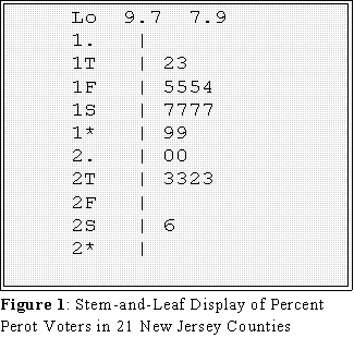
- Example: Percent voting for Perot in 21 New Jersey counties: Here are the raw data:
- The counties are numbered consecutively.
Table 1
Percent for Perot, 1992
New Jersey, by County
No |
Percent for
Perot |
No |
Percent
for
Perot |
| 1 |
17.6 |
12 |
15.8 |
| 2 |
12.9 |
13 |
17.1 |
| 3 |
20.4 |
14 |
15.5 |
| 4 |
17.6 |
15 |
19.3 |
| 5 |
20.1 |
16 |
13.0 |
| 6 |
19.0 |
17 |
26.0 |
| 7 |
9.7 |
18 |
17.4 |
| 8 |
23.1 |
19 |
22.0 |
| 9 |
7.9 |
20 |
11.4 |
| 10 |
23.6 |
21 |
23.8 |
| 11 |
15.5 |
|
|
- Figure 1 shows a stem-and-leaf display using this type of labeling.

- Another example:
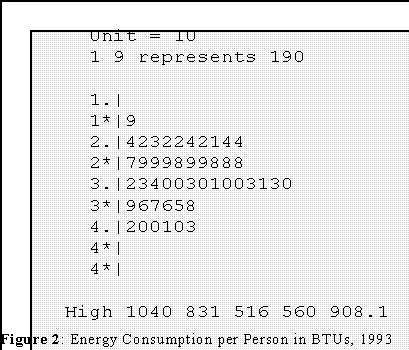
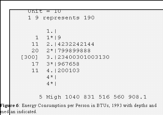
- Per capita energy consumption in 50 states in BTUs in 1993.
- The raw data are in the data section of
of the course page.
- We can use this example to demonstrate other topics.

- Interpretation: Note that the shape of the distribution is "symmetric" (that is,
about half of the observations are above average and half below; see later.)
and "bell-shaped"
- There are 5 "outlying" or large values. Since they are considerably above or
larger than the rest of the data, we give them their own stem called "High"
- DEPTHS: COUNTING UP AND DOWN A BATCH
- Overview: in order to calculate some summary statistics we need to order the
numbers in a batch (that is, arrange them from lowest to highest) and then count
relative positions.
- A depth is a number that indicates a position from the bottom or top of a ordered
batch.
- To see how depths can be useful, it is sometimes easiest to rank all of the leaves on
each row (stem) from lowest to highest.
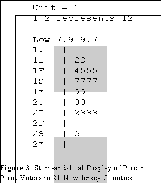
- Example: the Perot data once again.
- This is the same display as Figure 1, but the leaves have been arranged in
order starting with the lowest at one end and the highest at the other.
- That is the first "row" is written 7.9 and 9.7 instead of the reverse (9.7
and 7.9)
- The leaves on the second and third rows have also been ordered from
lowest to highs.
- At the top, the leaves descend in order.
- Ordering the numbers this way is not necessary but does help us calculate order
statistics or statistics based on the order of the data points.

- Depth: a data point's position or place in the batch, counting from one end of the
scale or another.
- Example: consider the batch of ordered data 10 12 45 67 89 107
- The "depth" of 12, say, is 2 (because it is the 2nd score form the bottom); 3
is the depth of 45; and so-forth.
- In Figure 3, the "depth" of 7.9 percent is 1 because it is the first (smallest)
number from the bottom.
- At the other end, 26 is the maximum value: its depth is thus also 1 because it
is the first number counting from the top.
- Thus the depth of a number is how far it is from the low or high end of the batch,
which ever is closer.
- To locate the depth of a value:
- Rank order the data from lowest to highest or put them in a stem-and-leaf
display in which the leaves are sorted from lowest to highest as in the above
example.
- Count from the bottom or low end of the scale if the number is closest to that
end or count down from the top or high end if that's where the number is
closet to.
- The number's depth is its position.
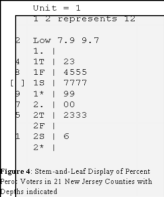
- One way to annotate a stem-and-leaf display is to write the depth of the leaves on
each stem row. In the previous example:

- Notice: that we count from both ends of the scale.
- Note too the brackets in the "middle" stem. This row contains the observation
that lies in the middle of the batch. Hence we mark it for special treatment.
- STATISTICS BASED ON POSITION:
- We can calculate statistics based on the depths, which really shows us the order.
- The statistics are the median (the "middle" value); the upper and lower hinges (the
"middle" value of the upper and lower halves of the batch); the upper and lower
eighths (the "middle" values of the upper and lower quarters of the batch); and so
forth.
- MEDIAN:
- Definition: sample median is the numeric value of a variable that marks the middle
of a batch of numbers in the sense that half of the observed values are below it and
half above. In other words, the median is the number that divides a batch of numbers
in half.
- Example: 10 20 30 40 50
- The median is 30 because half of the numbers are below, half are above 30.
- Calculation of the median:
- We use depths to find the median.
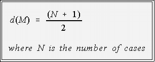
- If n is odd, the depth of the median is

- Example: if we have 21 cases, the median has a depth of:

- That is, the 11th value in the ordered batch is the median.
- Count down (or up) 11 cases and find the numerical value of
the median.
- Example, the depth of the median based on the 21 cases in
Figure 4 is 11. That is the median is the 11th number
counting from either the top or the bottom.
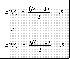
- If N is even, the median is the average of the two middle values:
- First, find the depths of the middle two values:

- Examples:
- N = 5: 103 120 135 194 1007

- Thus, the median is the value of the third observation: M = 135
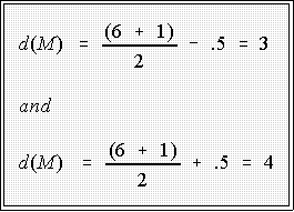
- N = 6: 103 120 135 194 1007 1200

- Thus, the median is the average of the 3rd and 4th values, namely the
average of 135 and 194.

- This suggests that a median will not always be an actual or observed data
point.
- Median Calculated From Stem-and Leaf Displays
- To find the median order the values of the stem-and-leaf display and find the
depths.
- If N is odd the median can be read directly from the stem and leaf display:
simply find the value associated with depth d(M).
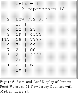
- Consider the Perot data: since N is odd, the depth of the median is

- Here is the stem-and-leaf display with the depths and median, 17,
indicated between the parentheses.

- If N is even the median will be the average of the values associated with
depths d(M)l and d(M)u.
- Example: energy consumption data

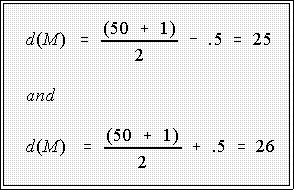
- The depths for the median, since N is even, are:

- Thus the median is the average of the 25th and 26th observations:

- Notice that the median is just the average of 300 and 300 or 300..
- Properties of the Median
- Appropriate for numeric data and order grouped data.
- Splits the batch (sample values) in half.
- The median is generally not equal to the "average" or mean (see below).
- Median is a RESISTANT measure of central tendency: that is, it is not
"influenced" by "outliers" or extreme values.
- Example:
10 20 30 40 50 M = 30 Average (mean) = 30
10 20 30 40 500 M = 30 Average (mean) = 120
- One has to order the data in order to calculate the median. So, if some
quantities are not known exactly, the median can still be calculated. Suppose,
for instance, that the highest per capita consumption of energy was known to
be above 1,000. The median can still be calculated since we only need to find
the number midway between the lowest and highest value without having to
know exactly what those values are.
- HINGES:
- The median divides the data into two batches with equal numbers. We can in turn
divide each of these sets in half.
- That is we can find the "median" of the "lower" batch and the median of the
"Upper" batch.
- These order statistics are called hinges.
- Example: consider this set of 9 numbers
6 11 17 19 22 30 34 49 67
- The depth of the median is just

- And the median is the 5th number from the top or bottom or 22.
- Hence 22 divides the batch in half.
- Each of these batches can be divided in half.
- The depth of the hinge is (formally):

- "The integer part" means ignore any fraction if there is one in the depth.
- That is, find the number or point that divides the lower and upper batches in
half. Example. for this case where d(M) is 5 the depth of the hinge is:

- So find the third number from the bottom in the lower batch and the third
number from the top in the upper batch. These are the lower and upper
hinges.
- 6 11 17 19 22 30 34 49 67
- The hinges are thus 17 and 34.
- Energy consumption example.
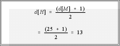
- The median depth is 25.5, which when used in the formula for the depth of the
hinge gives (don't forget to drop the .5 part)

- The lower hinge is the 13th number or rate from the bottom or 280 BTUs per
capita and the upper hinge is the 13th point from the top or 380 BTUs.
- THE MEAN:
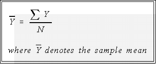
- As is well known, the mean is the "average" value in a batch of data. It is found by
summing the scores--summation is denoted by the Greek capital letter sigma, --and
dividing by N, the number of data points or cases in the batch:

- The sample mean is usually denoted with a bar over a letter.
- Do not be intimidated by the sigma sign. It simply means "add." The context in which
appears will usually make it clear what is to be added. For example, the notation
Yi means:

- Not that the mean is not a very "robust" or "resistant" indicator of central tendency,
since a few "extreme" cases can affect its numerical value. (See the example above.)
- This is one reason income is often reported as a median, rather than mean,
value. If everyone, except one or two millionaires, earns about $20,000, the
mean may suggest that average income is higher than most of us would think
were we to see the total distribution.
- A large discrepancy between the mean and the median suggests that the data
batch might be "skewed" in some fashion or that it contains a few "outlying"
values.
- NEXT TIME:
- Using the median and hinge to draw graphs of the distributions of variables.
- Box plots.
- Multiple stem-and-leaf displays and boxplots.

 Go to Statistics main page
 Go
to H. T. Reynolds page.
Copyright © 1997 H. T. Reynolds
