DEPARTMENT OF POLITICAL SCIENCE

AND

INTERNATIONAL RELATIONS

Posc/Uapp 815

LARGE AND SMALL SAMPLE MEANS TESTS

AGENDA:

Sampling distribution of the mean.
Another example of large-sample means test
t-test of means for small samples.
Difference of means test
Reading:

Agresti and Finlay, Statistical Methods, Chapter 6:

SAMPLING DISTRIBUTION OF THE MEAN:

Consider a variable, Y, that is normally distributed with a mean of and a standard deviation, s.
Imagine taking repeated independent samples of size N from this population.
Each time a sample mean, is calculated.
Statistical theory shows that the distribution of these sample means is normal with a mean of and a standard deviation.
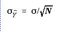More precisely, in case you are interested, this result stems from the so-called central limit theorem.

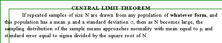
Notice that the expected value of the sample means equals the population value () but the standard deviation, called the standard error of the mean, is the population standard deviation divided by N.
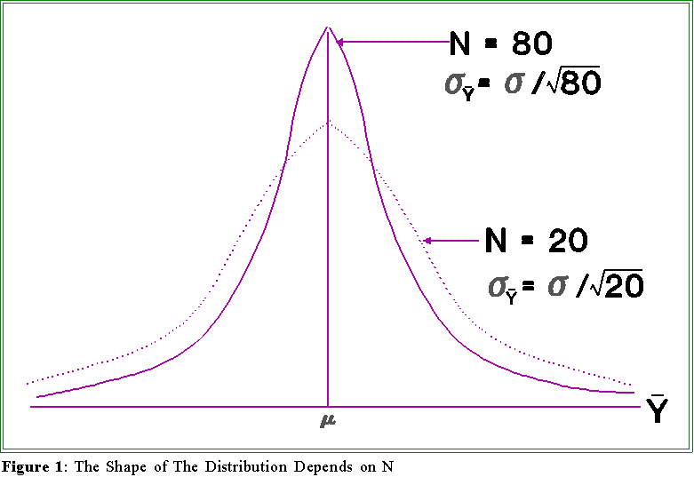
Here is a picture of one of the consequences of this fact. In the diagram, means have been drawn from some population (not necessarily normal). In the first instance, where N is 80, the sample means cluster rather tightly around the "true" mean (). This is because 80 is being divided into . In the second case, where the sample sizes are 20, the sample means are more spread around the true mean. That, of course, is because s is being divided by a smaller number and hence the standard error (i.e., standard deviation) is larger. Thus, the sample means in case 2 are more dispersed.

ADDITIONAL EXAMPLE OF MEANS TEST:

Here is still another problem; this time we can discuss it with less commentary. Go over it and if questions arise, be sure to ask them. Transportation has become a national problem. The Federal Highway Administration is studying different ways to merge automobiles onto high speed expressways and interstates. One project involved an experiment in Florida in which a series of display lights is used to tell drivers whether or not they are traveling at an appropriate speed to merge with the on coming traffic. It has been know from many prior studies that the average stress of drivers merging onto congested highways is 8.2 (measured on a 10-point stress scale where 10 means most stressed). In a sample of 200 drivers using the signal-light system, the average stress score was 7.6 with a standard deviation of 1.8. Is there any evidence that the system is reducing stress?
Hypothesis:

Research hypothesis: the system lowers stress so that for drivers using it < 8.2.
Null hypothesis: H₀: = 8.2 (The system does not lower stress.)
This is again a one-tailed test. The alternative (research) hypothesis suggests the direction in which we would expect to find the mean of drivers using the system.

Sampling distribution:

Since N is 200 use the normal distribution. If the null hypothesis is true then, sample means taken from this population will be normally distributed with mean 8.2 and standard error equal to sigma divided by the square root of 200. Since sigma, the population standard deviation is unknown we will estimate it with the sample standard deviation, 1.8.

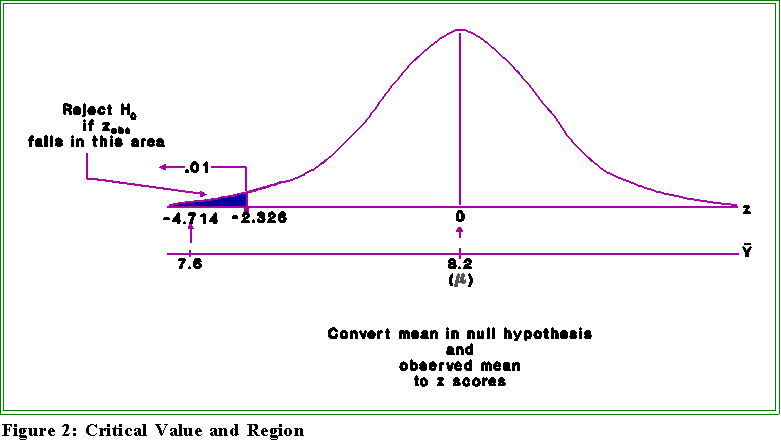
Critical region:

Let's use the .01 level: we want to make sure that our decision about H₀ is reasonable; that is, we don't want to commit a type I error (reject the null hypothesis when it is in fact true) because otherwise we would be instituting a system that really didn't work.
Thus, find the critical z that marks off the lower .01 proportion of the distribution. It turns out to be about 2.326. (See the diagram below.)

Test statistic:

Using the formula given above we find the observed z as:

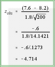
Thus, the observed z is -4.714

Decision:

Since the absolute value of the observed z is so much greater than the critical value, we reject the null hypothesis at the .01 level. That is there is only a very small chance that H₀ is true.

Interpretation:

Although the null hypothesis has been rejected the difference between drivers using the system of lights and all other drivers is relatively small. Therefore, one next has to ask if this difference has any practical significance. Will the light system, in other words, reduce tension enough to prevent accidents?

COMPUTER SOFTWARE:

If you have raw data, use MINITAB's Stat, then Basic statistics, then 1-sample z.
SPSS has a similar procedure.

t TEST OF MEANS:

Problem: Suppose it is known that the body weight at birth of normal children (single births) within the United States is approximately normally distributed and has a mean, , of 115.2 ounces. A pediatrician believes that the birth weights of normal children born of mothers who smoke regularly may be lower on average than for the population as a whole. In order to test this hypothesis, the doctor obtains the birth weights of a random sample of 8 children whose mothers are heavy smokers. The mean of this sample is 114.0 ounces with a standard deviation of = 4.3 ounces. Evaluate the pediatrician's hunch. (Taken from William L. Hays, Statistics for the Social Sciences, 2nd edition, p. 428.)
Hypothesis:

Null: H₀: = 115.2
Research: < 115.2

Note the mean, , here means the population average birth weight of children born to mothers who are heavy smokers.
The research or alternative hypothesis suggests a one-tailed test: birth weights equal to or greater than 115.2 will automatically lead to acceptance of H₀. It is only "smaller" birth weights, that is those less than 115.2 ounces, that will cast doubt on H₀. The only question is how small the sample weights have to be before one rejects H₀. Consequently, we will define the critical region as those sample results sufficiently below 115.2 to causes us to doubt the tenability of the null hypothesis.
If the doctor had no idea what the birth weights of children born to heavy smokers might be, we would reject the null hypothesis if the average sample birth weight were either much greater than 115.2 or much lower than 115.2. In this case we would construct critical regions at both ends of the sampling distribution, thereby creating a two tailed test.
But since the pediatrician specifies ahead of time an alternative hypothesis, we will stick with a one-tailed test.
Note finally that H₀ and H_A are mutually exclusive and exhaustive. That is, one and only one hypothesis can be true.

Sampling distribution:

Since N is small (or because we do not know the population standard deviation) we need to use a different distribution called the t-distribution.
The t distribution is really a family of distributions with each particular one depending on the sample size, N, or more exactly on the so-called degrees of freedom which is defined as:

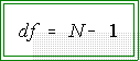
The degrees of freedom for this problem in which N is 17 is:

Each t distribution is roughly "mound" shaped: it looks a little bit like a normal distribution but is flatter in the middle and has more probability (area) in the tails. Nevertheless, the t distributions are symmetric around a mean of 0.
The t distribution is used just like the standard normal: the only exception is that one has to first calculate the degrees of freedom, a simple matter because the formula is so easy.
When the degrees of freedom are found and an appropriate level of significance (alpha level) is chosen refer to a table of t values.
A table of the t distribution is attached and one is also available in Agresti and Finlay, Statistical Methods

To use the table do this:

Find the row corresponding to the degrees of freedom.
Find the column corresponding to the desired level of significance and type of test (one-tailed or two-tailed)
The entry will be the critical value which will be compared to the observed value (see below).

Critical region and values:

This is a one-tailed test since only large sample statistics will cause us to reject the null hypothesis.
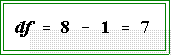
The birth weights of normal children are believed to be normally distributed. Furthermore, we are considering a sample mean based on a small sample (N = 8). Hence the appropriate distribution is the t distribution with 8 - 1 = 7 degrees of freedom.

Level of significance and critical region

Suppose we want to work at the .05 level of significance. That is, we set a = .05. In other words, we are willing to live with a probability of making a type I error (incorrectly rejecting the null hypothesis) of .05. We might pick this relatively "high" probability because even if we are wrong and mistakenly conclude that infants born to smokers have on average lower birth weights than normal babies in general, the "costs" of the mistake are not overly great. Advising people to quit smoking is sound advice for other reasons.
The sampling distribution, nature of the test (one-tailed), and sampling distribution determine the choice of a critical region. We need to consult a tabular version of the t distribution with 7 degrees of freedom and find the critical value associated with a critical region equal to a = .05.

The value shown in the t table is 1.895. This is found by looking in the 7th row (corresponding to 7 degrees of freedom) and the t_.050 column. (If we were using a two-tailed test at the .05 level, we would use the a/2 = .05/2 = .025 column.)
Figure 3 illustrates the distribution, critical value, and critical region.

The decision will thus be:

Reject H₀ if the absolute value of t_obs is greater than or equal to the absolute value of 1.895.
Otherwise fail to reject H₀.

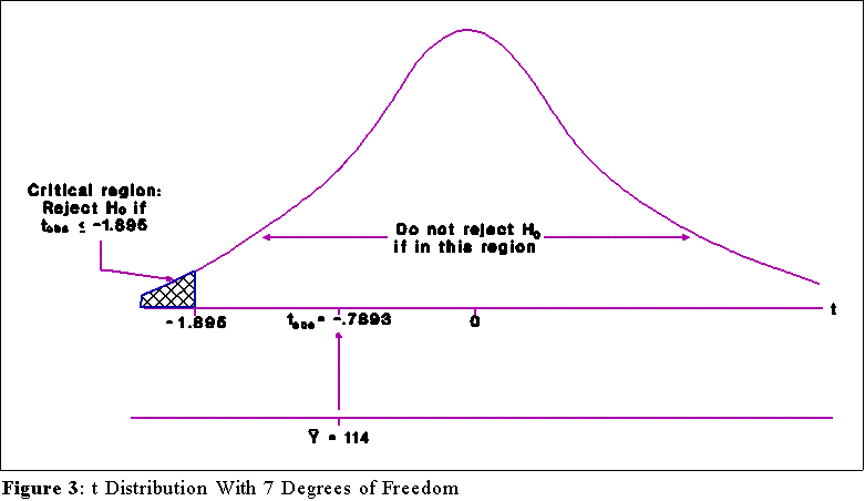
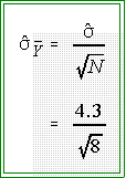
Sample statistic:

Since N = 8 and= 4.3, the observed t is:

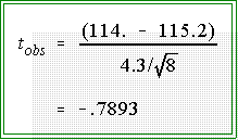
Note that the estimated standard error of the mean is given by the usual formula:

Decision

The absolute value of the observed t, -.7893, is not greater than or equal to the absolute value of the critical t. Therefore, we fail to (or do not) reject the null hypothesis.

Interpretation

Although the sample birth weights are lower on average than the population mean, we have to conclude that this discrepancy could have occurred by chance.
Personally, I would want a larger sample size.

The power of this test--the probability of finding an effect size greater than 0--is relatively low.

But we also have to keep in mind what a "meaningful" difference is. Even if the population mean for babies of smoking mothers is 115.2 - 114 = 1.2 ounces less than all normal babies, does this difference in weight put the infants at risk? This is, of course, a medical question. I raise it because, if N were large enough, we would have rejected the null hypothesis. To convince yourself of this point use the same data as presented in the problem, but assume that N is 10,000.

TWO-SAMPLE DIFFERENCE OF MEANS TESTS:

Paraphrased from Michael Oakes, Statistical Inference (New York: Wiley) pp. 4-5.
Testing hypotheses revisited: Suppose a researcher is interested in the effects of televised violence on children's behavior. She takes a random sample of 20 young boys and randomly assigns them to two groups. One group watches an especially violent episode of a children's TV program; the other sees a movie about a foreign culture. Then, the youngsters are observed at play. The investigator records the number of times a child behaves aggressively toward a large doll or play figure.
Suppose the investigator proposes the following substantive or research hypothesis. Children who view violence on television will tend to imitate those aggressive behaviors that are reinforce on the programs. Children not exposed to such violence tend to behave much less aggressively.
The statistical hypotheses can thus be stated this way:

H₀: m₁ = m₂
H_A: m₁ > m₂

where m₁ is the mean number of aggressive acts performed by the "population" of children who view violence on television and m₂ is the mean number of aggressive acts performed by the "population" of children who do not view violence on television.

If H₀ and H_A are mutually exclusive and exhaustive (as they are), then if H₀ is denied, H_A should be accepted. (The investigator seeks to deny H₀, or to nullify it. Hence, the term null hypothesis.)
Note that both H₀ and H_A refer to population parameters (that is, m₁ and m₂), but only sample statistics () are available.
It is important to note that a particular sample statistic (the difference between sample means, for instance) is only more or less likely given the truth of one of the statistical hypotheses. That is, we cannot say definitively on the basis of a sample whether H₀ or H_A is true. We can only make an inference.

Note also, that although I may occasionally be sloppy in my spoken vocabulary, we are investigating the probability of obtaining a sample result as large (or larger than) the one observed, given that the null hypothesis is true. Hence, if H₀ is true, we ask how likely is that we would observe a difference in aggressive behaviors of such and such magnitude.

Hypothesis testing rests on the idea that a particular sample statistic (once again in this case the difference between sample means) is but one instance of an infinitely large number of sample statistics that would arise if the experiment were repeated an infinite number of times. The differences between sample statistics would reflect two sources of variation: first the vagaries of random sampling from an infinite population, and second, if and only if the alternative hypothesis were true, the differences between the populations. Statistical theory demonstrates that by using information from the samples and by making a few assumptions, one can construct a sampling distribution of the difference of sample means. (One assumption is that H₀: ₁ = ₂ is true.)
More precisely, statistical theory tells us that if the assumptions are met, then the distribution formed by plotting the difference of two sample means over an infinite number of hypothetical replications would be bell-shaped and symmetric with mean equal to 0 and standard deviation (i.e., standard error) equal to.
More precisely, again assuming certain conditions hold, (e.g., H₀ is true) the standardized sample statistic

will have a t distribution with

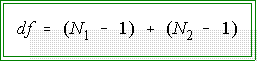
degrees of freedom, where the N's are the sample sizes of the two groups.

The observed t

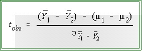
may take any value from minus to plus infinity. But the sampling distribution shows us the relative frequency of t_obs falling in any interval of the distribution

Although t_obs may theoretically take any value, it is clear that some are more likely or probably than others, if the null hypothesis is true. Thus, a statistical test rests upon the notion that the "truth" of a null hypothesis is called into question by some observed t values but not others.
This logic is exactly the same as used in testing a hypothesis about a single mean or a series of coin flips.

The only difference is that the sample t is now based on the difference of sample means and hence has a different standard error.

Notice that the expected value of the sample means equals the population value but the standard deviation, called the standard error of the mean, is the population standard deviation divided by N.
Here is a picture of one of the consequences of this fact. In the diagram, means have been drawn from some population (not necessarily normal). In the first instance, where N is 80, the sample means cluster rather tightly around the "true" mean (m). This is because 80 is being divided into s. In the second case, where the sample sizes are 20, the sample means are more spread around the true mean. That, of course, is because s is being divided by a smaller number and hence the standard error (i.e., standard deviation) is larger. Thus, the sample means in case 2 are more dispersed.

TWO-SAMPLE TEST EXAMPLE:

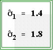
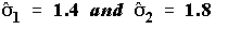
Let us, using hypothetical data, follow up on the previous example. Suppose the investigator finds that in the experimental group, the one exposed to televised violence, the average number of aggressive behaviors is 6.2 per hour (with a standard deviation of 1.4). The corresponding mean for the control group is 2.3 with a standard deviation of 1.8.
Hypotheses:

H₀: m₁ = m₂

Note: H₀ implies that m₁ - m₂ = 0

H_A: m₁ > m₂

Sampling distribution:

The difference of means based on N₁ and N₂ cases in each group will have a t distribution with degrees of freedom equal to

The mean of this distribution will be 0 and have a standard error equal to

Level of significance, critical region, and critical value.

For this problem we use a one-tailed test. Why?
Let's set the level of significance at the .01 level. That is, we want the probability of making a type I error (falsely rejecting the H₀ that the two types of children do not differ) to be 1 in 100.
Since we have 18 degrees of freedom (why?), we find from the tabulated distribution of the t statistic that the critical value is 2.552. (Why?) Thus, if the observed t (in absolute value) equals or exceeds 2.552, we will reject H₀; otherwise we will continue to accept it.

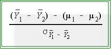
Test statistic

We now have to compute the sample test statistic. Part of the problem is easy. The null hypothesis specifies that ₁ - ₂ = 0. We can also easily calculate the difference in the sample means: 6.2 - 2.3 = 3.9.
Thus, the numerator of the test statistic (t_obs) is:

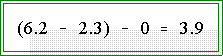
Remember m₁ - m₂ = 0

It only remains to calculate the standard error of the difference of means. Since we have only samples, we have to estimate this value. That is, we need to find

Notice the hat.

The formula for the estimated standard error of the difference of means contains two parts:

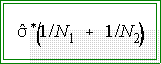
We next need the formula for It is:

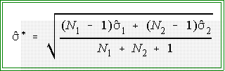
whereare the sample standard deviations of the two groups. That is:

Also, in this example N₁ and N₂ = 10. In general, however, the N's do not have to equal one another.

Given all of these parts the sample statistic is:

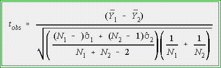
For this problem where N₁ = N₂ = 10 and the formula works out to:

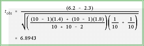
Decision

Since the absolute value of the observed t exceeds the critical value (2.552), we reject H₀ at the .01 level.

It seems likely that the two populations of groups differ with respect to their aggressive behavior. In other words, the "population" of children who watch televised violence are "significantly" more likely to act violently themselves than are youngsters who are not so exposed to this form of entertainment.

MISCELLANEOUS NOTES REGARDING TWO SAMPLE TESTS:

Software:

If you have raw data pertaining to two samples in different columns, you can use MINITAB's Stat, then Basic statistics, then 2-sample t to carry out the tests.

For the results presented above to hold we have to make several assumptions:

The two samples are independently drawn and random
Each N is less than 20. If the N's are large, the t statistic will be approximated by a z statistic. That is, for large samples use the z statistic.
The distribution assumes H₀ is true.
This method assumes that the two population standard deviations, s₁ and s₂ are equal. If this assumption does not hold, we need to adopt another procedure, but that topic will not be discussed here.

You can compare sample standard deviations by looking at box plots.

GENERAL REMARKS ABOUT HYPOTHESIS TESTS:

Some general points and propositions: these are intended to help you understand what significance tests do and do not tell a researcher or citizen.
What makes a result significant?

Significance tests have the form

Example: large sample test of mean:

Test of two means (large samples):

Note that these formulas contain two components:

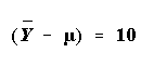
The numerator can be called (very loosely) the "effect size." It measures what is of substantive interest. For example, suppose the hypothesized mean of some population is m = 0, whereas the observed mean, is 10. The number 10 may or may not be a "large effect," depending on the measurement scale, the problem, and so forth. The point is that, all other things being equal, the larger an effect size, the more likely the test statistic will be found "statistically significant."
This is what we want or expect. After all, when someone says "My findings are significant," you no doubt infer that the person's has found a substantively large and interesting result.

The problem is that other factors affect whether or not the effect will be judged significant. In particular look at the denominator, the so-called standard error of the statistic under investigation.

Note, that again other things being equal, if the standard error is large, then the test statistic will be small.
Suppose. Consider two cases, one in which the standard error is 2 and one in which it is 20. In the first instance, the z statistic will be 5, which is highly significant (in the statistical sense); in the second case it is, .5, a non-significant value.
So we should ask what makes a standard error large or small. That takes us to the denominator.

Again loosely speaking, the standard error has the form:

That is, the standard error will be large or small depending on how large or small the population standard deviation(s) and sample size(s) are.

For a given standard deviation, the larger the N or N's, the smaller the standard error.
Example: imagine dividing a standard deviation of 20 by first N = 10. You get 2. Now divide it by N = 200; the result is .1.
To make the standard error small--and hence the test statistic large--all one need (for a constant standard deviation) is a relatively large N or Ns).
In fact, one can by increasing the sample size, make the standard error as small as one wants. Doing so will in turn make the test statistic large and hence significant.

To clarify the point, consider an investigator who, studying some phenomenon collects data on 20 cases. The person then compute the effect size which turns out to be 5. Suppose also the standard error works out to be 5. Then the z statistic is 1.0, which is not statistically significant. (Look it up.) But then suppose, another individual, working on the same problem but, having more money, samples 2,000 cases. Even if the effect size remains the same, as it could, the z statistic will be highly significant because the standard error will be small. Why? Look at either the general formula or the one for the test of a mean.
Further remarks. Consider this passage from the New York Times, which shows the need to balance "statistical significance" against substantive significance. The issue is the risk of having a heart attack after strenuous exertion or exercise.

The article underlines a couple of points

A risk of illness in one circumstance (a sedentary life style, for instance) may be many times the corresponding risk in another situation. True, enough.
But also it is important to examine the actual numerical estimates of the risks.
In this example, the risk of heart attack after exercise or exertion is greater for people who lead "sedentary" life styles, but the risk is still relatively small.
So, when formulating health policy, one has to have reasonable expectations about the consequences of making a recommendation. Suggesting that people exercise is good advice, according to these data, but those who do not follow it will not necessarily drop like flies.

From the New York Times, December 2, 1993, p. 18.

But he [Dr Curfman] noted that only about 5 percent of heart attacks occurred in association with heavy physical exertion; the rest occurred while the person was resting or performing moderate activities like driving a car, shopping, golfing...or raking leaves.

But he added, "So many heart attacks occur each year that even 5 percent is quite a large number." For example, the authors of the American study calculated that in this country at least 75,000 heart attacks a year, leading to 25,000 deaths, are related to exertion.

On the other hand:

Lest the new findings cause panic among those who must rush to catch a plane or change a tire, the Boston team noted that while the relative risk of suffering an activity-related heart attack could be very high, especially for habitually sedentary people, the absolute risk for any given hour of intense activity was actually very low. In other words, even a sedentary person is not very likely to have a heart attack within an hour of doing something strenuous like shoveling snow or digging up the garden.

How can we reconcile these comments and findings? The rate for a 50 year old man who does not smoke or have diabetes is one in a million during a given one-hour period. "If this man was habitually sedentary but engaged in heavy physical exertion during that hour, his risk would increase 100 times over the base line value, but would still be only one in 10,000," the Boston researcher wrote.

Estimation: most statisticians and many social scientists feel that it is more important to obtain "precise" estimates of population parameters than conduct tests of significance.

We will discuss the construction of confidence intervals, which help us guess the true value of a population parameter, next semester.

Test of null hypotheses are, as I have noted on several occasions, often not very informative since the researcher knows ahead of time that H₀ is not true.

Look in the tables of most published research, especially those presenting regression coefficients. Usually the estimated coefficients are listed in columns with stars or asterisks denoting those that are significant. By this the author means that the hypothesis that b = 0 is rejected. But usually we know this ahead of time. What do we learn, for example, from a test that finds a significant b between, say, crime and social standing?
Perhaps more impressive research would proceed along these lines: "Previous studies have found that the coefficient between X and Y is .25. Hence, I set the null hypothesis as b = .25. That may, or may not, be harder to reject. But if it is, the rejection may convey more information. And even if it isn't, we may learn more.

Go to Statistics main page

Go to H. T. Reynolds page.