DEPARTMENT OF POLITICAL SCIENCE
AND
INTERNATIONAL AFFAIRS
Posc/Uapp 815
TIME SERIES AND STATISTICAL INFERENCE

- AGENDA:
- Intervention analysis: simple interrupted time series model
- Basic ideas of statistical inference.
- Sampling distributions
- Reading:
- Agresti and Finlay, Statistical Methods, Chapter 6, pages 154 to 167.
- INTERVENTION ANALYSIS:
- The basic problem is to develop a model that succinctly shows the effect of an
"intervention."
- The dependent variable is a quantitative or numeric measurement taken at evenly
spaced time periods such as months or years.
- The "intervention" is conceptualized as an "event" or "policy" that in some sense
interrupts the series.
- See Class 21 notes for some hypothetical examples.
- The effects of the intervention can be modeled by counter
and dummy variables.
- Counter: a series of integrers (1,2,3,...) that identify time periods.
- Dummy variables.
- One can create a variable or set of variables to represent categories of a
non-quantitative factor.
- Suppose a variable has two categories such as male and female or before
and after an intervention.
- Select one category as a reference category. The choice can be made
arbitrarily but usually represents substantive interests.
- Example:
- X1 = 0 for before observations
and X1 = 1 for after observations
- Example:
- X1 = 0 for females
and
X1 = 1 otherwise (that is, for males)
- Example:
- X1 = 0 for South (that is, southern states or counties)
and X1 = 1 otherwise (that is, non-southern states or counties)
- Dummy and counter variables can be entered into a regression model by
themselves or along with other independent variables.
- A MODEL FOR A CHANGE OF SLOPE OR TREND:
- Here are some data pertaining to turnout--the percent of the voting age population
that voted--in congressional or "off-year" elections in the United States.
| Year |
Turnout |
| 1934 |
41.4 |
| 1938 |
44.0 |
| 1942 |
32.5 |
| 1946 |
37.1 |
| 1950 |
41.1 |
| 1954 |
41.7 |
| 1958 |
43.0 |
| 1962 |
45.4 |
| 1966 |
45.4 |
| 1970 |
43.5 |
| 1974 |
35.9 |
| 1978 |
34.9 |
| 1982 |
33.0 |
| 1986 |
33.5 |
| 1990 |
33.1 |
| 1994 |
36.0 |
- Congress passed the "Voting Rights Act" in 1965, right in the middle of this series.
Its goal was to protect every citizen's right to vote. Many have interpreted it as
landmark legislation that provide effective enfranchisement to African-Americans.
- An obvious question then is what effect, if any, did the legislation have on
turnout measured as the percent of the population old enough to vote who
actually did vote in congressional-year elections.
- In particular we are interested in changes in the turnout trend before and
after passage.
- We know that turnout has for a variety of reasons been declining
throughout the twentieth century. But one wonders if the law slowed or
reversed this downward spiral.
- Model:
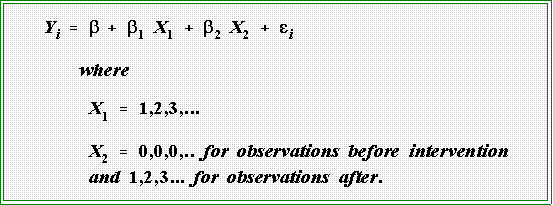
- Here's a simple model for measuring the law's effects on the slope or
trend.

- It's perhaps easiest to interpret this model or equation by first looking at
what is says for observations (years) before the intervention, that is, before
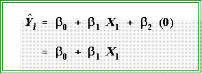
passage of the law in 1965. For those years X2 = 0 and the model reduces
to:

- Thus, the coefficients indicate the slope and intercept of the line before the
intervention.
- For the post intervention years, however, the second X does not drop out
and b2 measures the post-intervention change in the slope.
- Example:
- Here are the OLS estimates for the turnout data.

- Turnout increased very slightly before 1965 as indicated by the positive
slope of .704. But after 1965 turnout declined precipitously.
- EXTENSIONS:
- Note that the previous model is overly simplistic and would have to be modified
for both substantive and statistical reasons.
- We'll take up these extensions next semester.
- PROBABILITY:
- Here are some problems and questions:
- From "Rosencrantz and Guildenstern Are Dead" by Tom Stoppard.
Rosencrantz (Ros) and Guildenstern (Guil) are flipping coins:
- Ros: Eighty-five in a row--beaten the record
- Guild: Don't be absurd.
- Ros: Easily
- Guil (angry): Is that it, then? Is that all?
- Ros: What?
- Guil: A new record? Is that as far as you are prepared to go?
- Ros: Well...
- Guil: No questions? Not even a pause?
- Ros: You spun them yourself.
- Guil: Not even a flicker of doubt?
- Ros (aggrieved, aggressive): Well, I won--didn't I?
- Guil:...And if you'd lost? If they had come down against you, eighty-five times, one
after another, just like that?
- Ros (dumbly): Eighty-five in a row? Tails?
- Guil: Yes! What would you think?
- Ros:...Well....(Jocularly.) Well, I'd have a good look at your coins for a start!
- A lawyer has just called because she has been troubled by recent events at
the local courthouse where welfare fraud cases are being heard. Although
the proportion of females in the county is .53, she thinks that women are
under-represented on the juries dealing with these cases. Last week, for
example, only two out of 12 jurors were women? Is there any evidence, she
wants to know, of discrimination?
- The board of directors of a local charity (e.g., United Way) claims to be
unbiased. But a civil rights group points out to you that of 10 members
only 1 is black, even though blacks make up 15% of the community. Is
there any evidence of discrimination or is this composition a matter of
chance? They want your advice before taking the charity to court.
- The administration of the University of Delaware is concerned about the
dropout rate. They believe that if students saw their advisors more
frequently the dropout rate would decrease and hence are considering
measures that would make advisement easier to obtain. The reforms,
however, will be expensive to institute. Consequently, they undertook a
study in which every student was asked how often he or she saw an
advisor. The average (mean) number of visits was 12. Some months later a
random sample of 40 dropouts was interviewed during which time they
were asked how frequently they saw an advisor. The mean number of visits
for the sample of dropout students was 9.1. Is there any reason to believe
that the average number of visits to advisors among the dropouts is
significantly lower than the average number of visits for the student
population as a whole? Is there, in other words, sufficient evidence for
instituting an expensive advisement process?
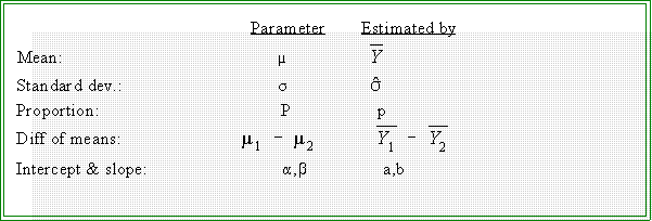
- Review of terms and concepts
- Population versus samples
- Parameters versus statistics
- See the following table:

- Note: the notation for the estimators of the intercept (regression constant)
and slope (regression coefficient) are often
 and
and  .
.
- Goals of statistical inference:
- Test hypotheses about population parameters
- Estimate the magnitude or value of population parameters
- A simple example:
- Question (hypothesis): Suppose you are flipping coins with someone. A
reasonable question is: is the person honest?
- How should one "operationalize" the notion of honesty?
- The question really asks: is the probability of getting a "head" on a single
flip of a coin 1/2 = .5? The hypothesis suggested by the question, in other
words, is that P[heads] = .5 More formally,

- H0 is called a null hypothesis
- In a series of , say, 10 flips of a coin how likely is it that a person will get 9
heads?
- In order to answer this question you have to decide two things:
- What is "likely"? That is, what is your definition of likely or
probable and conversely what is your definition of improbable?
- Given this definition, you then have to decide what outcomes--what
number of heads in 10 tosses--that you will consider probable and
what number you will believe to be improbable.
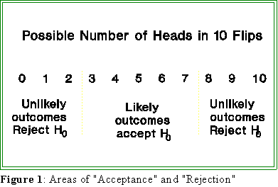
- Stated another way you have to form a mental picture like this:

- Next, observe an actual set of ten tosses and count the number of heads.
- Finally, make a decision using the guidelines presented above: if the
observed number of heads fall in the region of rejection because this result
is improbable, then reject the hypothesis (P[heads] = .5) and conclude that
the coin is biased, the person is crooked, etc.
- If, for example, someone tosses a coin 10 times and obtain 9 heads then
you might suspect that the hypothesis of honesty is untenable.
- STEPS IN TESTING A HYPOTHESIS:
- Problem: A drug manufacturer claims that its anticoagulant drug is 80 percent
effective (that is, the probability of preventing clots is .8) based on thousands of
trials with primates, mice, and even human volunteers. The FDA has sent you data
pertaining to 8 randomly selected individuals in a Veterans hospital, only 2 of
whom were helped by the drug. If the "true" proportion of "success" is .8, how
likely is it that you would observe only 2 out of 8 successes? Could this result have
occurred by chance, thereby supporting the manufacturer's claim or is it such an
improbable result that you are led to doubt the drug's efficacy?
- Research hypothesis: The FDA believes that the probability of success is less than
.8 (that is, P < .8).
- The null hypothesis is: H0 = .8
- A null hypothesis always asserts that a population parameter equals a
specific number, frequently zero but in this case .8.
- Sampling Distribution:
- Loosely speaking, a sampling distribution is a theoretical distribution that
shows the relationship between the possible values of a given sample
statistic (e.g., sample number of successes) based on N cases and the
probability associated with each possible value.
- Thus, if we know a sampling distribution for a statistic, if we have a sample
of N cases, if we have an actual observed value of the statistic, and if we
have a particular null hypothesis in mind, we can tell how likely the
observed result is. Based on this information, we can decide whether or not
to accept the null hypothesis.
- In this case the statistic in question is simply Y, the number of successful
treatments in N trials.
- Hence, in this case we have N = 8 and have observed Y = 2.
- An appropriate sampling distribution will tell us the likelihood of getting 2
or fewer successes in 8 independent trials given that the null hypothesis is
true.
- The material that follows is designed to show where this particular sampling
distribution comes from.
- To find the probability of Y successes in N trials given that the probability
of success is P use this formula:

- The term P(Y,N,P) means the "probability of getting Y successes in N
trials given that the probability of success is P.
- As we have already seen, the symbols N! and Y! mean "factorial"
N! = N(N - 1)(N -2)(N -3)....For example, 8! = (8)(7)(6)...
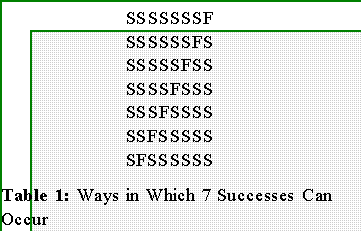
- The first part of the equation represents how many ways 7
successes can be obtained in 8 trials. For example, these are the
ways we can obtain 7 successes in 8 trials:

- In the table S denotes a success and F a failure. In the first line, 7
successes are obtained on the first 7 trials. But this is not the only
way to get seven successes. The second line shows, for example.
that 7 successes can be obtained by getting 6 in a row, then a
failure, then another success.
- The number of these patterns is given by the first part of the equation; that
is,

- The second part of the equation gives the probability of getting Y
successes in N trials if the probability of success is P. This probability must
be multiplied by the number of ways of getting Y successes (see above).
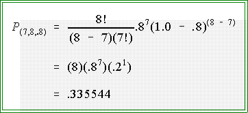
- Example: suppose the probability of getting a "success" is P = .8. In addition,
suppose we want to know the probability of getting Y = 7 successes in N = 8 trials
or attempts. According to the formula the probability is

- Note that 8! = (8)(7)(6)(5)(4)(3)(2)(1); that 7! = (7)(6)(5)(4)(3)(2)(1); and
that 1! = (1). Thus, the first part of the equation reduces to 8, since 8!/7! =
8 which in turn is divided by 1. See the listing above.
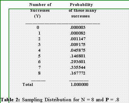
- By letting N = 8, P = .8, (1 - P) = .2, and letting Y equal successively 0, 1,
2, 3,...we get this sampling distribution.

- You can get this table from MINITAB by opening the session window and typing
at the MTB> prompt

- Parts of the Sampling distribution
- Decide which sample outcomes (e.g., number of successes) are so
improbable to you that should one of them occur, you will not accept the
null hypothesis. This is called the critical region.
- The cutoff value--the value at or below which you reject the null
hypothesis--is called the critical value.
- In this case let it be 4: hence if you observe 4 or fewer successes in
8 trials you will reject the H0 that the true probability of success is
.8.
- NEXT TIME:
- Dissection of sampling distribution.
- Tests of means and proportions.

 Go to Statistics main page
 Go
to H. T. Reynolds page.
Copyright © 1997 H. T. Reynolds
