DEPARTMENT OF POLITICAL SCIENCE
AND
INTERNATIONAL AFFAIRS
Posc/Uapp 815
VARIOUS REGRESSION MODELS

- AGENDA:
- Two variable regression example
- Multiple regression
- Multiple regression model
- Partial regression coefficients
- Reading:
- Agresti and Finlay, Statistical Methods, Chapter 10, pages 356 to 371
- Read for understanding. There is a great deal of useful and important
information in these pages.
- TWO VARIABLE REGRESSION:
- Lets explore the
"State Expenditure"
data in a bit more detail.
- Recall that the variables are:
- Per capita state and local public expenditures ($)
- Economic ability index, in which income, retail sales, and the value of
output (manufactures, mineral, and agricultural) per capita are equally
weighted.
- Percentage of population living in standard metropolitan areas
- Percent change in population, 1950-1960
- Percent of population aged 5-19 years
- Percent of population over 65 years of age
- "WEST"
- West is a "dummy" variable codes as: Western state (1) or not (0)
- First let's try to explain variation in states' ability index. We might hypothesize, for
example, that the more "metropolitan" or urban the state, the higher its index. The
presumption is that urbanization is related to retail sales, income, and the like.
- We'll try to do the regression in class, but in case we can't or the screen is not clear,
here is the estimated regression equation.

- The interpretation is straight forward.
The estimated regression coefficient
indicates that a one percent increase in urbanization (percent living in
metropolitan areas) is associated with about a third of a point increase in the
ability to pay index.
- There is, in other words, some evidence of a positive correlation.
- How much? The measures of goodness of fit are R2 = .158, suggesting that
a small part of the variation in the expenditure ratio is accounted for or
explained by the independent variable.
- This is not an especially large value.
- Similarly, the simple correlation coefficient, r = .398, is relatively
small.
- This finding raises several possibilities:
- There simply isn't much of a relationship.
- The modest or small correlation is due to or caused by some
unmeasured or excluded factor.
- One or both variables are not properly measured.
- A combination of these.
- We will try to improve the fit by adding another variable to the analysis.
- See the section on multiple regression
- Additional examination of the data: analysis of residuals
- Recall that errors in the regression model are supposed to be random.
- One way to check this assumption and to also find ways to improve the fit is
to examine the residuals.
- The residuals are:

- There is a residual for each data point. They are rough estimators of the error
terms and as such should be randomly distributed above and below zero.
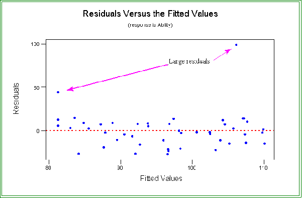
- A common technique is the residual plot of the observed residuals plotted
against "fitted" or predicted values.
- That is, one can plot the pair:
ei
versus

- See the attached figure for an example.
- The full version of MINITAB's regression choose plot residuals in the
options box.
- In the Student version, check both the "fits" and residuals boxes in the
Storage list. Then go to plot and plot residuals as the dependent
variable and "fits" as the independent factor.
- The points should be scattered more or less at random.
- In this example we see that for the most part the residuals are scattered above
and below zero, as they should be, but also note that two residuals are quite
large.
- Hence, we should investigate these cases more thoroughly.
- The two cases are numbers 42 and 47.
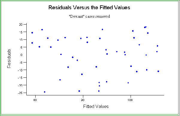
- For example, if one or both of the cases are removed the fit improves.
- The new estimated model is: = 79.3 + 0.308 X, where X is percent
in metropolitan areas.
- The R2 is now .283.
- And the residuals now appears more random scattered about the
"zero" point.
- See the attached graph.
- Now suppose we want to add additional factors to see if we can better understand
variation in the dependent variable.
- MULTIPLE REGRESSION:
- We'll return to the state expenditure data but first here are some additional data.
- This information pertains to birth rates and population growth in several countries.
PROJECTED POPULATION INCREASE
Nation |
Birth rate
X1 |
Death rate
X2 |
Life expectancy
X3 |
GNP per
capita
X4 |
Percent projected
population
increase
Y |
| Bolivia |
42 |
16 |
51 |
510 |
53.2 |
| Cuba |
17 |
6 |
73 |
1050 |
14.9 |
| Cyprus |
29 |
9 |
74 |
3720 |
14.3 |
| Egypt |
37 |
10 |
57 |
700 |
39.3 |
| Ghana |
47 |
15 |
52 |
320 |
60.1 |
| Jamaica |
28 |
6 |
70 |
1300 |
21.7 |
| Nigeria |
48 |
17 |
50 |
760 |
71.6 |
| South Africa |
35 |
14 |
54 |
2450 |
40.1 |
| South Korea |
23 |
6 |
66 |
2010 |
21.1 |
| Turkey |
35 |
10 |
63 |
1230 |
36.9 |
- Questions:
- What explains variation in Y, projected population increase?
- What are the "individual" effects of the independent variables?
- Are any of them redundant?
- How well does a linear model as a whole fit the data?
- What policy implications, if any, does the model contain?
- MULTIPLE REGRESSION MODEL:
- There is a single dependent variable, Y,
which is believed to be a linear function of K
independent variables.
- In the example, K = 4 because there are four independent
variables, X1, X2,
X3, and X4.
- The general model is written as:

- Sometimes the model is written equivalently as:

- The particular model for the
comparative population data is:

- Interpretation:
- Systematic part:
- Note first that I am now
writing the constant term as beta
instead of alpha. This is just a common convention.
- The regression parameters,
b's, represent the effects of each
independent variable on Y when the other variables in the
model have been controlled.
- Thus, b1,
is the effect of X1 when the other X's have been
controlled.
- The reason the word "controlled" appears is that the
independent variables themselves are interrelated. Changing
the value of, say, X1, not only changes Y but might also affect
X2 which in turn impacts on Y. To see the "pure" or
"uncontaminated" effect of X1 on Y we need to hold the other
X's constant.
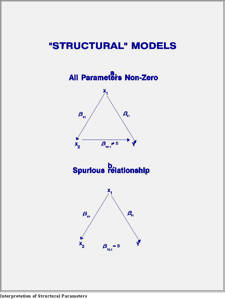
- A path diagram may help explain. Consider the models in the attached
figures.
- Note: that multiple regression coefficients are often written with the
dependent variable, Y, first, an independent variable (X2, for example) second,
and any variables that are being controlled after the dot. Thus, Y2.1 means the
coefficient between Y and X2, when the X1
has been (statistically) held
constant.
- In the first diagram (a),
Y depends on both X1 and X2.
Changing X1 will affect
the value of Y, even if we hold the other independent
variable (X2) constant.
Similarly, if we change X2, Y changes also. The "arrow" indicates that the
beta "connecting" Y and X2 is non-zero.
- Thus, the regression procedure produces partial or controlled coefficients
which means that Y changes 1 units for a one-unit
change in X1 when X2 has
been held constant.
- Note that direct linkages are indicated by arrows; an arrow represents
the presence of a non-zero beta coefficient.
- Now look at the second figure (b).
Here X2 is not connected directly to Y.
But there is an indirect relationship: as X1
varies so do both X2 and Y. If we
measured only the X2-Y relationship, we might be
tempted to conclude that
the two variables are related. But when X1 is added to the model, this
relationship disappears.
Why? Because Y2.1 gives the partial or controlled
effect: when X1 is controlled there is no
effect of X2 on Y.
- This latter case is an example of spurious correlation, examples of
which we have discussed several times during the semester.
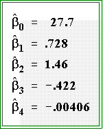
- To return to the population data, the estimated coefficients from the data set are:

- The estimated model is thus:

- The first parameter is the constant: it is the value of Y when all X's are zero.
- Note that as before the regression coefficients are measured in the
units of the dependent variable.
- Hence, they cannot be directly compared with one another.
- That is the coefficient for X2 is numerically twice the size of
the one for X1, but this does not mean it has twice the
importance or is twice as strongly related.
- The first regression parameter,
 ,
means that Y increases .738
units for a one-unit change in X1 when X2, X3,
and X4 have been held
constant.
- The second parameter is interpreted in a similar way: Y changes by
1.46 percent for every one-unit change in X2, assuming that X1, X3,
and X4 have been held constant.
- Note that partial regression coefficients are statistical means of
physically holding variables constant. In other words, observational
analysis limits our ability to manipulate variables so we compensate by
making statistical adjustments.
- Random error part:
- The ei in
the model once again represents random error--that is, random
measurement error in Y (but not X's) and the idiosyncratic factors that affect
the dependent variable.
- The observed Y scores are thus composed of the effects of the X' plus a
random error. The random error is not observed independently; it is estimated
from the residuals.
- Ideally, these errors really are random: they have an expected value of zero,
a constant variance (their variation does not change with changes in X's), they
are independent of the X's, and they are serially uncorrelated.
- OLS ESTIMATION:
- As before assume that estimates
of the parameters have been somehow obtained. With
these estimates we can obtain predicted values of Y's as in, for example:

- Since there will usually be a difference between predicted and observed Y's, we can
take the difference to get residuals or estimates of errors:

- The mathematics of OLS leads to estimators of the 's that minimize the sum of these
errors. In other words, the parameters are chosen such that

is a minimum.
- Note that OLS assumes that the assumptions about errors mentioned in class 19 notes
hold.
- MULTIPLE REGRESSION COEFFICIENT, R2:
- As in two-variable regression, TSS measures the total variation in Y, the dependent
variable.
- This total variation can be partitioned
into two main parts, as before:

- These quantities can be obtained from the ANOVA table part of the regression
results.
- The measure of fit is R2, also
called the coefficient of determination is
also defined as:

- ANOTHER EXAMPLE:
- Let's return once more to the state expenditures data.
- We'll continue to use the data with two cases
(numbers 42 and 47) removed.
- Suppose in addition to percent of state population
living in metropolitan areas we add
another variable, rate of population growth.
- Now we have two explanatory factors
and the estimated regression equation is

- The betas are the "partial" regression coefficients: they tell how much Y
changes for a one unit increase in an X when the other X has been held
constant.
- The estimated regression equation is:
79.2 + 0.307 X1 + 0.006 X2, where X1 is
percent living in metropolitan areas and X2 is growth.
- We have a regression constant, 79.2, and
two partial regression coefficients.
- A one percent change in "metropolitan" is associated with a .307 point
increase in expenditure capacity when growth has been held constant.
- One might think of the coefficient this way: suppose we looked only
at those states having the same or a common growth rate. Then b =
.307 would measure the correlation between percent urbanization and
expenditure capacity.
- Note that is value is only slightly different from the one obtained with
two variable regression: .338 when no cases have been deleted and
.308 when the two states are removed.
- So adding another variable, growth, does not change the previous
results.
- But in many instances adding or subtracting a variable from a model
will alter the sizes of coefficients. Doing so can even change their
signs.
- The other coefficient is interpreted in the same way. It measures the
relationship between growth and capacity after urabanization (X1) has been
held constant.
- Fit.
- Adding a second variable does not really improve the fit of the model since R2
is .283, which is exactly what the previous result was.
- Note. This is such a strange result it is interesting. Normally, adding
a variable will increase the multiple R, however slightly.
- PROGRAM PACKAGES:
- Multiple regression analysis is performed with the same software procedures used in
the two variable case.
- Add independent variables to the list of factors or predictors.
- One can and should obtain residual plots. Do so in the same way as before: use
plotting options or store residuals and fitted values and then plot them.
- NEXT TIME:
- Intervention (time series)
- Dummy variables.
- Statistical inference
Figures
Residual Plots


Multivariate Models


 Go to Statistics main page
 Go
to H. T. Reynolds page.
Copyright © 1997 H. T. Reynolds


