DEPARTMENT OF POLITICAL SCIENCE
AND
INTERNATIONAL RELATIONS
Posc/Uapp 815
MORE ON DISTRIBUTIONS

- AGENDA:
- The binomial distribution
- Bernoulli trials
- Sampling distributions
- Reading:
- Agresti and Finlay, Statistical Methods, Chapter 4, pages 94 to 99; pages
187 to 191.
- PROBLEM:
- Here's a hypothetical policy issue that Agresti and
Finlay suggest on page 191.
- I have embellished the example a little bit.
- Suppose you are an Equal Employment Office investigator. A group representing
women complains to you that a local construction firm refuses to hire women,
even for positions requiring no particular gender traits. As a matter of fact, they
argue, the company recently expanded and took on 10 new employees, only two of
which were female. They take this result as evidence of discrimination and want
you to take the matter to the judicial system.
- So, you call the company president who says of the complaint, "Look, we don't
discriminate. We hired the people more or less randomly, since the positions don't
require any specific skills. It just so happens that only 2 women were selected.
That's just a chance result that provides no evidence of discrimination."
- Assuming that women constitute 50 percent of the members of the potential labor
force in that area, would you accept the president's explanation? If not, why not?
- NOTATION AND TERMS:
- First some terms, notation, and background.
- Think of hiring 10 employees as flipping a coin 10 times. Each time the "coin"
lands one of two results can occur, a female or a male.
- Such random or experimental process that can produce one of two possible
outcomes (male or female) is called a Bernoulli process.
- Suppose the process is repeated N
times and you are concerned with Y, the
number of occurrences of a particular type, such as the number of females in N
draws or "flips."
- Moreover, suppose the probability
of getting one of the two outcomes is p.

- According to the axioms and rules of probability, if an experiment can
result in just two outcomes, M or F say, and the probability of getting M is
p, then the probability of getting F, the other type, is 1 - p =q,
because p +
q must equal one.
- Example: if the probability of getting "heads" is .5, then the
probability of getting "tails" is 1 - .5 = .5
- In this instance if men and women are equally represented in the labor
force, then the probability of selecting a woman by chance (p) presumably
equals .5, as does the probability of drawing a man (q).
- Now, suppose Census Bureau data indicate that in fact men and women are
equally represented in the potential population of workers from which the
company draws its employees.
- Given this information can you make a reasonable judgment about the company's
hiring practices?
- THE BINOMIAL DISTRIBUTION:
- Recall the discussion of probability distributions: in this context a distribution pairs
scores or values of a variable with the probability of their occurrence.
- We drew a simple diagram to illustrate the idea.

- A distribution, which a mathematical expression (equation) "creates,"
associates values of a variable, such as Y or the number of occurrences of
something, with the corresponding relative frequency, proportion or
probability of those values.
- We saw an example in previous notes.
- For a variable that is normally distributed the normal probability
distribution function pairs values of Y with probabilities.
- This distribution has the properties we discussed ad
nauseam before.
- Example: values relatively far from the mean, say 2
standard deviations, occur with less probability than
those that are only, say, standard deviation from
the mean.
- Perhaps we can use these ideas to address the discrimination charge raised
earlier.
- Binomial distribution:
- Given N "trials" or experiments, each of which can result in just one of two
possible outcomes, the probabilities of which are p for the first type of
outcome and q for the second, the probability of getting exactly Y
outcomes of the first type and N - Y outcomes of the second is given by
the binomial distribution:

- The term N! means "N factorial" and is defined as

- Hence, Y! means Y times Y-1 times Y-2...times 1.
- At this point it is not essential to understand all of the equation or
function's details, although they are relatively straightforward.
- In word, the function says that given N "trials" or samples from a population in
which the probability of getting an outcome of a particular type is p and the
probability of the other type is q = 1 - p, the probability of obtaining Y outcomes
of the first type is P(Y).
- In the present case, we have N = 10 (10 people were picked); the probability that
anyone of them is female is supposedly p = .5; the probability of getting a male is q
= .5.
- We assuming that all of the drawings from this population are
independent of the other selections.
- That is, the chance of drawing a female stays the same for each selection.
- Furthermore the possible results or outcomes of these 10 draws are 10 males, 9
males 1 female, 8 males 2 females...10 females.
- The distribution provides the probability of getting any of the these results,
assuming that p = .5 and that the selections are independently drawn at
random.
- That is, successively substitute Y = 0, Y = 1, Y = 2 and so on into the
formula"

- If we successively insert the possible values of Y into the equation, we can
find the probability of getting that many females in 10 draws or selections,
assuming that the draws are made randomly and independently from a
population in which the probability of selecting a female is .5.
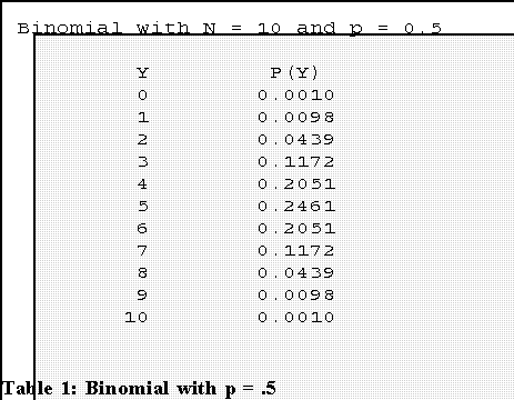
- Here are those probabilities

- That is, the probability of getting 0 females in 10 random selections
with the probability of drawing a female on any draw is .0010; the
chance of getting just one female is .0098; the probability of 2
females out of 10 (given that the proportion in the population is .5)
is .0439.
- What these results show is that if the company really selected employees at
random from a labor force consisting of half men and half women and if
they only hired 2 females, then it accomplished something rather unusual
for the chances of this result are less than 5 in 100.
- AN ALTERNATIVE EXPLANATION:
- Suppose that in fact the company's selection process purposely or inadvertently
favored men over women so that the chance of drawing a male was .7 and a female
.3.
- Note again: p + q must equal 1, since we are dealing with a Bernoulli
process. (That is, only one of two things can happen on any trial or attempt
or drawing.)
- In these circumstances the formula becomes:

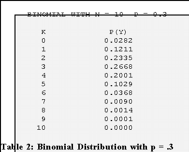
- If we substitute all the possible values of Y into this formula, we get

- Now we see that Y = 2 occurs fairly frequently or the probability that Y =
2 is fairly large, namely .2335.
- We would expect that a random drawing from a population in
which the proportion (or chance of a getting female) is .3 would
result in exactly 2 women to occur about a quarter of the time.
- That's a fairly probable result given all the conditions specified. It is
certainly more probable than if the conditions specified originally
held.
- So we might conclude that the company is in fact discriminating.
After all, it obtained an "unusual" result under the hypothesis of
fairness but an understandable one under the hypothesis of
discrimination.
- This line of thinking underlies hypothesis testing that will be covered soon.
- SAMPLING DISTRIBUTIONS:
- So far we have dealt with two types of distributions:
- Empirical or frequency: it shows the number of cases or observations
actually observed for each value (or intervals) of values of some variable.
- We noted that the shape of these distributions can take many forms
such as bell shaped or skewed to the right or left.
- Probability: it gives the expected probability of observing various values or
intervals of values, given that some set of conditions is true or holds.
- So if a random variable has a probability of .3 of being between,
say, 100 and 105, then an empirical frequency distribution of 1,000
cases should have about (1,000)(.3) = 300 cases in that interval.
- It won't contain exactly 300 observations because of
chance.
- The binomial and normal distributions are examples: they show the
probabilities of various scores.
- Sampling distribution.
- A sampling distribution is a particular kind of probability distribution. Or
more exactly, it's a particular application of a probability distribution.
- Example:
- Before going into any more detail consider this case: I asked each of you to
draw a random sample of 10 counties from the "population" of American
counties and to obtain a sample mean for these 10 cases.
- Consequently all 33 of you collected sample means that were estimators of
the true or population mean, which by the way was 7.33.
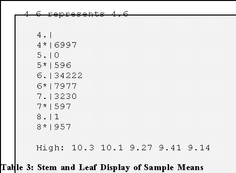
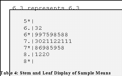
- The table below shows a stem-and-leaf plot of these 33 estimates.

- Thus, someone's estimate base on N = 10 counties was 10.3; another
person's estimate was 10.1 and so forth. Note that people's estimates ran
as high as 10.3 and low as 4.6, even though the true value is 7.33.
- Hence there was variation in the estimates: most were somewhere in the
middle in the range, say, of 6.5 to 7.5. But may estimates fell above or
below those values.
- We conclude that if one person (or a group of people) takes repeated,
independent samples from some population
having some parameter, theta , of
interest, the estimates of that parameter can vary widely.
- The estimates follow a distribution that depends on the size of the
samples, N, the form of the population distribution, and the value of the
parameter.
- Another example, the distribution of sample means when N = 100 was

- Note that again the estimates vary: some are above 7.33; some are below.
- So once again they are distributed. This time, however, the distribution is
based on samples of size N = 100, so the estimates don't vary as much as
in the previous instance where N = 10.
- Definition: a sampling distribution is a probability distribution that shows the
relationship between possible values of a sample statistic such as
 based on a
sample of N and the probability of those values given that various conditions hold.
- Example: sample means based on N cases drawn from a population with
mean = mu will be distributed in a particular way.
That distribution is called
the sampling distribution of the mean.
- See Agresti and Finlay, pages 99 to 100.
- Note that Tables 3 and 4 are not sampling distributions: they are empirical
distributions that I created to illustrate a point. A sampling distribution is a
mathematical equation.
- NEXT TIME:
- Some final remarks on distributions
- Explaining variation: relationships among variables

 Go to Statistics main page
 Go
to H. T. Reynolds page.
Copyright © 1997 H. T. Reynolds
