The Normal Distribution

1. AGENDA:
1. The normal distribution.
1. Interpretation of the normal distribution function.
2. Area under the normal curve
3. The standard normal distribution



2. THE NORMAL PROBABILITY DISTRIBUTION:
1. See the notes from the previous class.

1. THE NORMAL DISTRIBUTION:
1. One can think of the area under a normal "curve" as equaling 100% or 1.0, depending on whether one wants to talk about a percent of an area under the curve or a proportion of the area under the curve.
1. Areas under the curve can also be interpreted as probabilities.
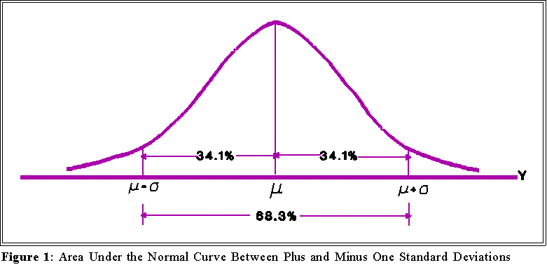
2. The area within plus one and minus one standard deviation of the mean constitutes about 68 percent of the area under the curve:

1. The area within plus and minus two standard deviations of the mean constitutes about 95 percent of the area under the curve (see Figure 2):

1. Hence, one can interpret the value of the standard deviation by reference to the normal curve. If a variable is distributed normally, then approximately two thirds of the population will lie (i.e., have scores) within plus or minus one standard deviation of the mean; about 95 percent will be within plus or minus 2 standard deviations of the mean. To see what this mean use MINITAB to calculate the mean and standard deviation of a normally distributed variable (use the stem command to see if the variable approximates a normal distribution). Then add and subtract 1 standard deviation to the mean. About two thirds of the cases should lie between these numbers.

1. USING AREAS UNDER THE CURVE TO ANSWER QUESTIONS:
1. The last point raise interesting and important questions.
1. How much of the area lies above three standard deviations from the mean?
2. How much lies between 0 and +1.5 standard deviations?
3. How many standard deviations above the mean marks the point which encompasses 49 percent of the area?
2. Here is a different question:
1. Suppose one believes that a variable Y has a normal distribution with a mean of 0 and a standard deviation of 10. An observation is drawn at random from a population of Y values and its score turns out to be 50. Does this observation (Y = 50) cast any doubt on the supposition. In other words, does getting a value of 50 from a population that supposedly has a mean value of 0 surprise you?
3. We can't answer these questions without more information.



2. THE STANDARD NORMAL DISTRIBUTION:
1. Since the normal curve is really a family of curves, each depending on a specific mean and standard deviation, statisticians use a single distribution, the standard normal distribution, to answer these types of questions.
2. Areas under the standard normal distribution have been tabulated and presented in the form of a so-called standard normal or z-table.
3. A standard normal distribution has a mean of 0 and standard deviation of 1. (That is, = 0 and = 1.) Areas under this curve--that is, the curve of the normal distribution with mean 0 and standard deviation of 1--have been extensively tabulated and appear in every statistics text.
1. The tables are called z tables. One is attached.
4. A z-table shows the percentage of the area under the curve--that is the percentage of the distribution--that lies between the mean and any specified number of standard deviations from the mean.
5. Example:
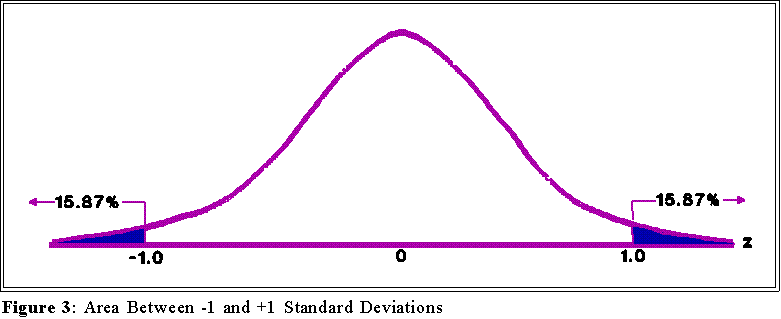
1. In a standard normal distribution how much area lies to the left of one standard deviation above the mean? Look in the column marked "z" and find 1.0. In the column labeled "second decimal place" find .00. The entry in the corresponding row and column is ..1587 This means that 15.87 percent of the area under the curve--15.87 percent of the distribution--lies below 1.0 standard deviation.
2. Since areas under a normal curve can be interpreted as probabilities or frequencies, we can think of .1587 as saying: "if a variable has a standard normal distribution, the proportion or of cases that will have values below one standard deviation from the mean (0) is .1587." Or, "the probability that a case lies 1 or more standard deviations above the mean is .1587."
3. Since the distribution is symmetric, the value .1587 also suggests that the proportion of cases lying below -1.0 is .1587
4. Figure 3 provides a picture:

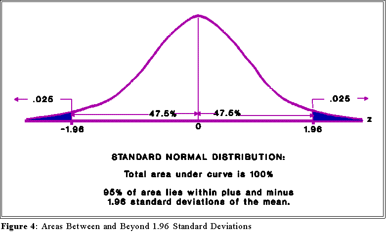
1. Look now in the z-value columns to find 1.96. (Use the 1.9 row and .06 column.)The corresponding area is .0250 which indicates that 2.5 percent of the distribution lies 1.96 standard deviations above the mean. (Also 2.5 percent lies below -1.96 deviations.)

1. The total area lying beyond +1.96 and -1.96 is:

1. Thus, 5 percent of the area is beyond plus and minus 1.96 or |1.96| standard deviations standard normal distribution.
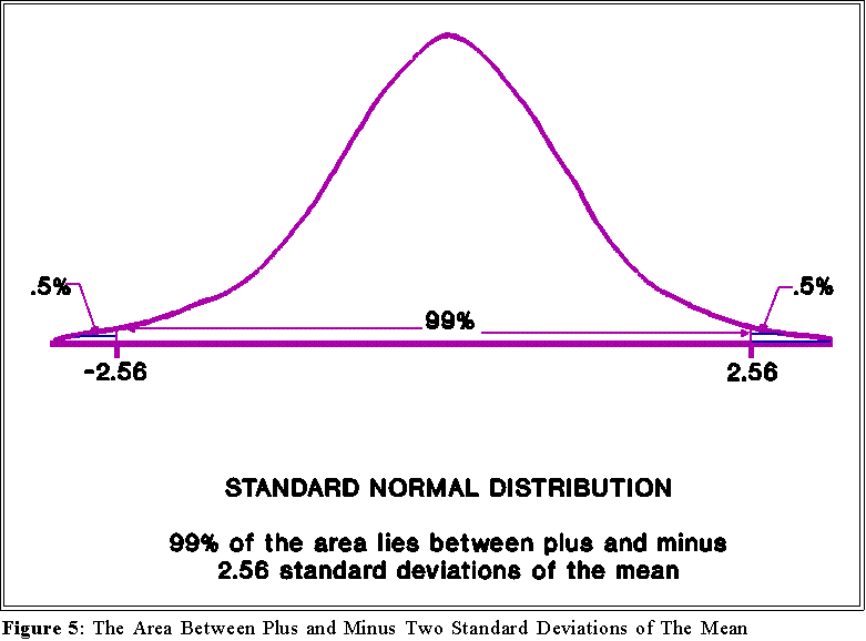
1. Look in the body of the table and find .0052. What standard deviation corresponds to this percent of the area? The answer, found by looking at the corresponding z columns, is 2.56. The usual interpretation applies: by going 2.56 standard deviations above (or below) the mean we define .5 percent of the area of the normal curve.

1. The total area beyond plus or minus 2.56 standard deviations is thus:

1. Figure 5 illustrates the point.

1. Using pictures and logic like this we can find the area corresponding to any two points along the z scale.
1. Example:
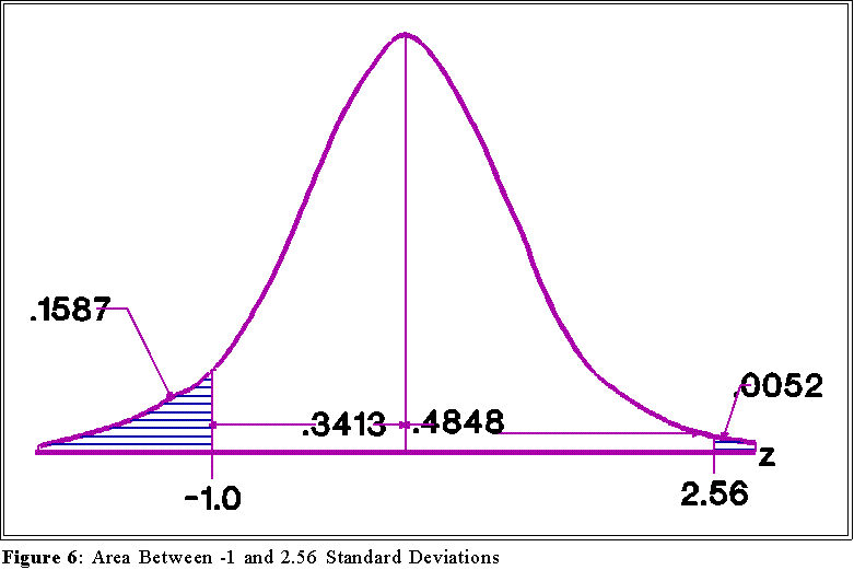
1. What is the area below -1.0 and above +2.56 standard deviations of a standard normal curve?
2. First draw a picture (see Figure 6):

1. We know from the table that .1587 proportion of the total area lies beyond -1.0. Furthermore, we know than .5 proportion of the area lies below 0. Thus by subtraction the area between 0 and -1.0 must be:

which we have seen before.

1. Similar reasoning shows that the area between 0 and +2.56 is:

1. Add these two areas together to get the total area between -1.0 and +2.56:

1. Looking at the picture we can see that the area lying above +2.56 and below -1.0 is:

1. Problem to work on: what proportion of the area under a standard normal curve lies between +.5 and +1.96 standard deviations? Use the methods outlined above to find the answer: draw a sketch of the normal curve. Label the points .5 and 1.96 along the z axis. Using the attached table find the areas beyond .5 and beyond 1.96. Then subtract these areas to find the amount between .5 and 1.96.



1. STANDARDIZED OR Z SCORES:
1. To use the standard normal distribution we have to change raw data to "standardized" data.
1. Remember the standard normal distribution has a mean of 0 and a standard deviation of 1.0, but we usually deal with different measurement scales where, for example, the mean might be 500 and the standard deviation 25. Thus, we wouldn't know from the table how much of the area is in the interval from, say, 463 to 589.
2. But we can find out by changing raw data to "standardized" or z scores.
2. To convert the data follow these steps:
1. Find the mean, , and standard deviation, of Y, the variable of interest.
2. To convert a particular raw score to a standard or z-score use the formula:

1. z is called a standard value, a standardized value or a z score. They are all the same. z is obtained from the original data by subtracting the mean of the original data and dividing by the standard deviation.
2. Examples:
1. Suppose we have a batch of data with a mean of 90 and a standard deviation of 10. What is the z score corresponding to a raw score of 100?

1. Suppose now the data are such that the mean is 1053.72 and is 105.69. What is the z score or standardized value corresponding to Y = 1950.18?

1. z scores may be negative as this example illustrates: the mean equals 55.7 and the standard deviation, , is 6.8. What is the z score for a raw value of 46.5?

1. NEXT TIME:
1. The standard normal distribution underlies hypothesis testing so we will explore it in more detail.

Go to Statistics main page

Go to H. T. Reynolds page.

Copyright © 1997 H. T. Reynolds