In a previous section, Michelson interferometer was described as a tool for determining wavelengths accurately.  A closer look at the behavior of this device shows that the entire spectrum emitted by a polychromatic source (or transmitted by a sample) can be measured accurately and quickly from its output.  The Michelson interferometer is used in virtually every modern infrared spectrometer. 

        The electric field exiting the Michelson interferometer is the sum of the electric fields that passed through the two (fixed and moving) arms of the device, here described as cosine waves of wavevector, k,

                                       

where z1 and z2 are the paths through the arm 1 and arm 2, respectively.  One way to write the irradiance, E, is as the time-averaged square of the electric field (scaled by the appropriate constants).

                                                 

The irradiance is the signal that would be recorded at a detector or observed by your eye.  The physical interpretation of the above equation is that detectors cannot respond as fast as the oscillations of a light wave, so they time average (integrate) the signal over the period , the detector response time.  The sign of the electric field also is not detected; E is squared.  The output of the interferometer can now be derived.

                                

Using algebra and trigonometry,

             

The rapidly oscillating terms (those containing ω) vanish because sinusoids always average to zero when τ>2π/ω.  The intensity output is thus a cosine wave that oscillates with the path difference Δz.  We can define E0=cε02E02 and rewrite this expression to emphasize that the intensity is a function only of Δz:

                                                             

This function is plotted in Fig. 7A with E written as an intensity, I.  Since intensity cannot be negative, it makes sense that the cosine wave is offset by one.  The Michelson interferometer has effectively reduced the oscillation frequency of the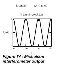

light signal (around 1014 Hz) to an arbitrarily low frequency that determined by the velocity of the mirror.  k/2π is the frequency in wavenumbers, which are the units typically used in infrared spectroscopy.

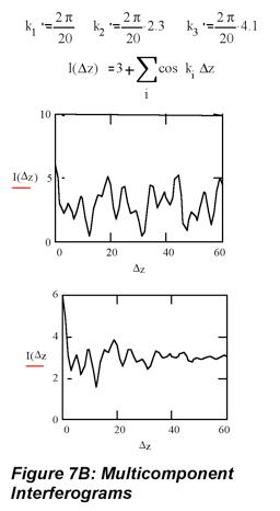
        The equation for E(Δz) given above applies to a single frequency beam of wavevector k.  In an interesting spectrum there are multiple frequencies (and therefore, wavevectors).  Intensities are additive, therefore, E(Δz) is a sum over all wavevectors, k.

      

This summation is a cosine Fourier series, a function whose mathematical behavior is well understood.  The Fourier series relates functions of conjugate variables (remember p (momentum) and x (position) in quantum mechanics), in this case Δz and k. E(Δz), the interferogram, is measured experimentally.  The spectrum is E(k), which is the intensity associated with each wavevector, is calculated from E(Δz).  The Fourier transform allows calculation of the spectrum, E(k), from the experimentally measured interferogram, E(Δz).

       A few examples are given here to illustrate how E(Δz) (the interferogram) is related to the spectrum.  Consider first a spectrum that has three infinitely narrow frequency components at arbitrary multiples of k.  The interferogram, shown to the right in Fig. 7B-1, has a periodic pattern reflecting the combination of three frequency components.  The corresponding spectrum, (not plotted) assuming the interferogram was collected over a long mirror distance, has three infinitely narrow, unit high peaks at k1, k2, and k3.  The Fourier transformation, which will be detailed later, calculates the coefficients (1, 1, and 1) of the oscillations (k1, k2, and k3) needed to reconstruct the interferogram, E((Δz). Next, in Fig. 7B-2, consider a spectrum that has the same three frequency components, but now with some discernible (non-zero) bandwidth.  The interferogram now decays as well as oscillates.   Experimentally, the interferogram is acquired by the data acquisition system until the interferogram has decayed to the point where the signal contains an intolerable fraction of noise.  Because all the frequencies in the spectrum are monitored simultaneously at all points in the interferogram, FT spectroscopy provides a substantial improvement in signal-to- noise ratio as long as the noise superimposed on the spectral signal is frequency independent.  This is called the multiplex advantage.  Similarly, the ability of the interferometer to analyze wavelengths without using slits to separate them leads to the throughput advantage.  Finally, the availability of very accurate wavelength calibration from the interference fringes of reference lasers improves the accuracy of the spectra that are measured.  These advantages motivate the broad use of interferometry in spectral measurements. All measurements don’t end up being improved by Fourier transformation, but many do. 

Fourier Transform Basics

        The Fourier transform is one of the most widely used mathematical tools in the physical sciences.  It describes the relation between fluctuating signals measured as a function of time (time domain) and their spectra, which reveal the relative amplitudes of the oscillations (frequency domain) comprising the signals.  We’ve seen that a Fourier transform relation exists between optical path length and wavenumber in the Michelson interferometer.  A Fourier transform relation between space and "inverse space", also is used to interpret solid state structures from x-ray diffraction patterns, but time-frequency are th set of conjugate variables we will focus on here.

        Any function in the time domain can be expressed as a Fourier series, that is a combination (sum) of harmonic oscillations

                           

where T is the acquisition time of the signal.  The time domain signal is represented as the function f(t); it is sometimes called a waveform.  The cosine Fourier transform of f(t) is

, φ(ω) is the phase of the cosine at ω.  In turn, f(t) is the inverse cosine Fourier transform of

.  If the waveform is expressed as a combination of sines, the sine Fourier transform of f(t) is

.  If the waveform is represented as a combination of cosines and sines (remember that eiωt = cos(ωt)+isin(ωt)), f(t) is the inverse complex transform of

.  The complex transform will be discussed further later in this section.  Each f(t) and 

combination (cosine, sine or complex) is called a Fourier transform pair.  (Plain variables represent time domain functions and capped variables represent frequency domain functions.) In the complex case, the inverse transform is algebraically simple and the waveform has a simple form in terms of the transform:

                                                       

where Nk is the number of frequency points in the transform. Equations 7.7 and 7.8 (a and b not shown) are written as summations rather than integrals because integrals apply to infinite, continuous functions, whereas spectral data are finite, discrete sequences. (The coefficient 1/Nk becomes 1/2π when f(t) is an infinite periodic sequence.  There will be more on using discrete transforms in the Numerical Fourier transforms section.)  A shorthand notation often used for the Fourier transform operation is FT, and for inverse transform, FT-1.  Thus,

                                                   

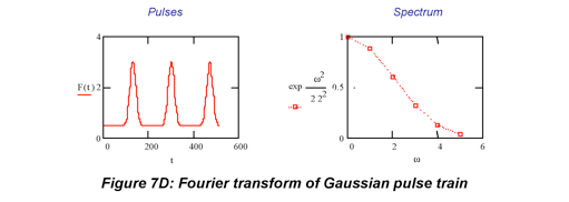
        There is an inverse relation between the widths of the functions f(t) and

.  A short pulse (time) has a wide spectrum (frequency).  Conversely, a pure cosine wave extending infinitely in time has an infinitely narrow spectrum (transform).  You encountered this relationship in quantum mechanics. The Heisenberg uncertainty relation, Δt*ΔE>h/2πc, states that one cannot know simultaneously the precise duration of a wave and its energy (or alternatively, an electron’s location and momentum).  This principle arises directly from Fourier transform relations because quantum mechanical entities behave like waves.  One decreasingly common illustration of this in daily life is the interference of spark sources on AM radio reception.  If someone turns on a power supply in the lab no matter what AM station is on, you hear the spark (static) because the spark (a short pulse in time) has a broad frequency spectrum. One of the simplest functions to transform is an infinite Gaussian function.  Its Fourier transform also is a Gaussian function, but in the frequency domain.  The Fourier transform relation between the widths of infinite Gaussians in the time and frequency domains is also very simple: σtσω=1.  This equation clearly shows the inverse relation between time domain and frequency domain functions.  While this simple relation (σtσω=1) only applies to Gaussians, it is generally true for any pair of transforms that σtσω=constant. 

        Consider the following example of the practical utility of this Fourier transform property.  If a fast electronic pulse is to be amplified and measured, one must ensure that the detection equipment responds quickly enough to measure the pulse without distortion.  Since it is convenient to think of the signal acquisition rate as a frequency (units are inverse seconds), we can describe detector performance using frequency limits and bandwidths.  So when you go to purchase detection electronics, you immediately find that the speed of a device is normally described by its frequency behavior.  An amplifier that has a response that drops significantly above 1 MHz, such as a typical operational amplifier, is useless for amplifying pulses that have widths much narrower than 1 μs (1 MHz=1/10-6 s).  Specification of the frequency at which the output drops to half its maximum value is a common performance parameter for an amplifier.  The amplifier bandwidth, the range of useful operation frequencies, is a common alternative.  The wider the amplifier bandwidth (frequency), the shorter the width of the signal (time) it will amplify.  Interactive web applets demonstrating these relationships are available (click here for example).

Fourier Transforms of Library Functions

       The most important property of the Fourier transform is its linearity. This means that the Fourier transform obeys a strict set of rules, specifically:

                                       

This means that whenever we can describe a new waveform as a multiple, combination or convolution of simpler functions whose transforms we know, we can compute the transform of the new waveform.  (There will be more on convolution later; for now think of it as a special type of vector multiplication in which the features of both vectors appear in the product.) Consequently, it’s useful to learn the transforms of a small number of simple functions that appear often in the context of spectral measurements.  We will use these functions as a kind of library for analyzing new waveforms. 

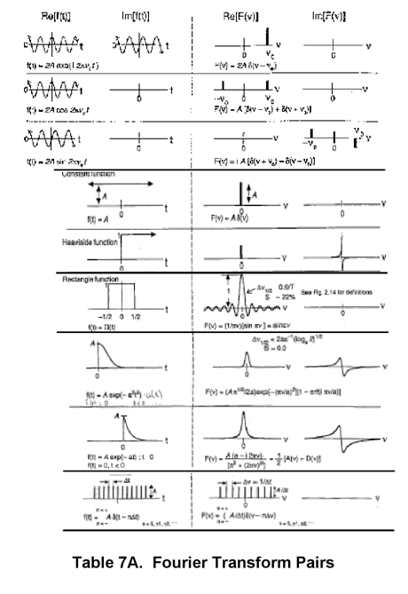
        One of the simplest functions to transform is Acos(ω0t); it has a single point in its spectrum (considering only the positive frequencies).   A sequence with a single non-zero point is a Dirac delta function.  In this case, the transform is represented as Aδ(ω−ω0), where ω0 is the location of the non-zero point on the frequency axis.  In Fig. 7C below, A is 22.68 and ω0 is 25.  There is an identical peak at ω0=-25 that is not shown here.  Notice that the Dirac function is also the transform of constant functions.  Remember a constant corresponds to a harmonic (cosine, sine or exponential) that has zero frequency.

         Adding cosine waves that have neighboring frequencies in the interferogram produces spectral bands that have a finite width in the transform.  This is illustrated in the following example, where the frequency components are weighted by a Gaussian function.  Again, the negative frequencies are not shown in Fig. 7C, but the left half of the spectral profile would be identical to the right, forming a Gaussian spectral profile.  (In fact the focus on the frequencies near zero in the figure obscures the fact that the transform consists of a train of pulses just as the waveform does.)

                                               

Since the inverse Fourier transform of a frequency domain Gaussian is a time domain Gaussian, the interferogram that generates this spectrum must consist of Gaussian profiles as well.

        It is interesting to see how frequency components combine to make familiar shapes.  For example, the rectangle or window function and the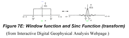

sinc function are a transform pair.  Adding cosines of similar frequency (within the window) will produce a waveform that is reinforced at zero (on the time axis) but decays quickly with time as it oscillates because of the ‘destructive interference’ of cosines of different frequency. 

        A similar function that is also important in spectroscopy is the square wave.  For example, lock-in amplifiers, which are electronic devices used to improve detection in many spectrophotometers, essentially multiply the instrument output by a “train” of square waves (See Figure 7F). For example in absorbance measurements, mechanical chopping of the source signal imposes a square wave on both the reference (incident) and sample (transmitted) signals.  This translates the signal to a frequency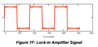

range that is not subject to drift and other low frequency noise to the extent that steady-state measurements are. The lock-in amplifier is used to operate the detector at the chopper frequency. The reference signal for the lock-in amplifier is generated by placing a small light-emitting diode on one side of the chopper and a photodiode on the other side.  The detector uses this signal to track the intensity changes produced by the chopper. A square wave is built from the odd harmonics of the chopper (fundamental) frequency, ω in Equation 7.12, (approximately 1/180 s ~ 0.006 Hz in Fig. 7F):

                                           

but it is also a periodic rectangle function, so the transform of the square wave is a sinc function that shows the relative importance of the harmonics of ω to the signal (see Fig. 7E). In the absorbance spectrometer electronic bandpass filters are used to isolate the chopper frequency in order to convert the measurement to a constant intensity.

Other important functions in spectroscopy include the Heaviside function, H(t-t0) which is zero (off) until some time t0 when the measurement starts, the exponential decay, f(t)=e-at, which describes the dissipation observed in many properties as random processes relax perturbed states and the comb function, which is a sequence of evenly spaced Dirac pulses.  The table at right depicts the Fourier transform pairs of the library functions that have been described so far.   

        Now we will use the library function concept to help us analyze what happens to a square wave (lock in amplifier signal) when it is improperly filtered electronically.  Consider the common example of low-pass filtering, where the square wave is passed through an RC (resistance-capacitance) filter with a time constant that is too low to capture all the signal features, as often happens because the frequency range of instruments is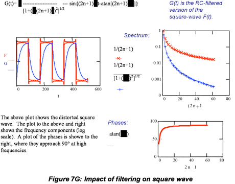

limited.  A low pass RC filter attenuates the frequency components by the factor [1/1+(ωτ)2]1/2, where τ=RC. In other words the filter multiplies the square wave transform by these attenuation factors (one at each frequency) and shifts the phase of each sine contributing to the square wave by ϕ(ω)= tan-1(ωτ), resulting in a highly distorted square wave when ωτ is sufficiently large. The question is ‘what is the shape of the distorted waveform?’  Fortunately, the attenuation factor is the transform of one of our library functions, the exponential decay, e-t/τ.  So we can predict that the sharp edges of the square wave will be distorted to exponentials by the filter.  Fig. 7G (blue trace) shows that this is indeed the case. The filtered square wave is the first signal discussed here for which phase is an issue.  The components of the filtered signal have real and imaginary components, which produce non-zero phases.  The next section explores such cases further.

Complex representations of Fourier transforms

In cases where the time domain signal is neither perfectly even nor perfectly odd (as all of the previous examples except the filtered square wave have been) both sine and cosine Fourier coefficients are required to describe f(t) in the frequency domain. For example, in interferometry, when the mirror alignment is not perfect the interferogram becomes asymmetric around the zero retardance point.  (Notice in Marshall & Verdun, App D that symmetric functions have only cosine transform coefficients.  This is because symmetric functions are even.)  Attempting to compute  from the asymmetric f(t), with the simple cosine transform produces a product

                                                   

where

is the amplitude of the Fourier coefficient and φ(ω) is the phase (we shall discuss these terms further shortly), rather than the transform . So any odd function will have a cosine transform for which the phases are not zero and transformation yields the product

. It is clear that this situation is not optima

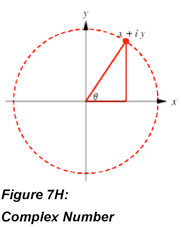l and Equations 7.7a, and 7.13 are inconvenient in this case because there is no way to separate the phase information from the coefficient information.  It is always important to know both

and

because both are needed to reconstruct the entire transform.  This is why we use complex Fourier transforms; they allow us to determine the transform coefficients and phase separately.  After a short review of complex number representations, we will see how they are used in Fourier transformations.

        The imaginary number, i, is the square root of negative one, i.e., (-1)1/2. (Sometimes (-1)1/2 is represented by j to avoid confusion with the current.) Complex numbers have both a real and imaginary part: z=a+bi.  The function Re extracts the real part of a complex number, while Im extracts the imaginary part:

                                                  

.

One way to think about complex numbers is as the components of a vector stopped at some point as it travels around a circle of radius

. (I think this reflects the central role stargazing and astronomy have played in the development of our mathematics.) With this picture we also know the angle the vector makes with the x axis.  In the picture it is θ, in our notation it is

                                                           

This means we can re-express z using Euler’s formula:

                                               

       Now back to Fourier transforms.  We use Euler’s formula to combine cosine and sine transforms into a single function:

                                              

The real part of the complex transform is the cosine transform and the imaginary part of is the sine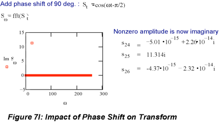

transform.  So the complex Fourier transform separates a function into even and odd components. Even functions, which can be represented by sums of cosines, will have only real numbers in their complex Fourier transforms. Odd functions, which are represented by sums of sines (cosines shifted by π/2), will have only imaginary numbers in their complex transforms (see Table 7A).  A function comprised of cosines shifted in phase by anything but an integer multiple of π will have a complex transform.

        The key to understanding the impact of the odd components on the interferogram transform is a second form of the complex Fourier transform of f(t) (see Eq. 7.7c for the first).  We can write any function as a sum of the product of harmonics and an explicit phase term:

                                            

where

is the amplitude of the combined cosine and sine coefficients.  Technically the above expression is the inverse transform of f(t). (FYI: The inverse transform has the same form as the transform, but with the sign in the exponential changed.  The term exp(iωt) is the "complex conjugate" of exp(-iωt).) The transform of f(t) is

               

In this treatment the cosine transform of the asymmetric interferogram in the frequency domain is

.  Remember, the reason we’ve rewritten the transform is to separate the coefficient and phase information.  The phase can be calculated from the complex transform components

                       

where real coefficients are given by

and the imaginary by

. In this form, the phase can be removed from the amplitude using simple trigonometry:

                           

Marshall & Verdum call the amplitude the magnitude, M(ω), others call it the power spectrum. Clearly, it is analogous to |z| in Equation 7.15. 

        Let’s reconsider the RC circuit using complex transforms. We know (from physics) that the charge in an RC circuit decays exponentially in time, consequently the frequency response of a low-pass filter can be described by taking the Fourier transform of a single-sided exponential decay.  Using f(t) = exp(-t/τ, τ=RC) (only for t>0), the complex Fourier transform is

                                     

It is not easy to see, but the filtered square wave is the convolution of the original square wave and the exponential decay that characterizes the filter. The sharp parts of the square wave rise and fall exponentially because passage through the filter attenuates the real and imaginary high frequency (fast) signal components by (1+ωτ)-1 and +ωτ/(1+ωτ), respectively. 

A second example of this kind of qualitative analysis of Fourier transformation comes from considering the transformation of a single frequency interferogram for which the length of mirror travel is i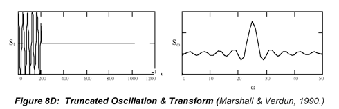

nsufficient.  The acquisition of the interferogram is stopped before the oscillation is completely acquired.  This is tantamount to multiplying the time domain signal by a rectangular window function.  Consequently, the Fourier transform of this incomplete interferogram is the convolution of the transform of the oscillation (a Dirac pulse) and the transform of the window (a sinc function).  This is illustrated above and discussed further in Section 8.