STATISTICAL ANALYSIS

After the data preparation is complete and a working data set is stored in a permanent SAS data step, analyses may be performed with comparatively simple programs. the data= option works on every SAS procedure. It tells the procedures to read data from a SAS data set named to the right of the equal sign. Each of the exercises in this section illustrate its use.

Exercise: Preliminary analysis -- Income Means by Sex and Race

As preliminary analysis, run the means procedure with a class statement identifying race and sex. First, start a new SAS session. In a UNIX terminal window, type --

     sas &

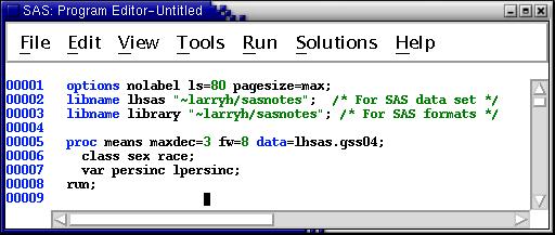
Enter the following program into the Program Editor --

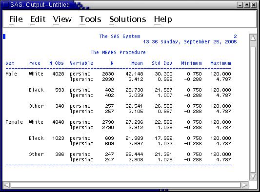
Submit the job and view the output. It shows the average annual income (persinc) and average of the log of annual income (lpersinc) by the six categories resulting from crossing the two genders with the three race categories. (The GSS does not report detailed racial breakdowns.)

This short program illustrates four options intended to make the output easier to decipher --

1. nolabel on the options statement: This option prevents all procedures from writing the variable labels to the output. In this example, the labels take up so much space that the output from the means procedure wraps onto more than one line for each variable, making it noticably less convenient to read.

2. pagesize=max on the options statement: This option makes the page length very long. SAS still starts a new page for each new procedure, but output for each procedure generally will contain no page breaks. Page breaks are useful for printing, but they make it difficult to compare different parts of the output in the Output Window. The difficulty is due to long sections of blank lines that pad the bottom of each page and to the fact that the Output Window jumps the display at the end of each page so that the top of one page and bottom of the previous page cannot be viewed at the same time.

3. maxdec=3 on the proc means statement: Calls for three digits to be printed to the right of the decimal point.

4. fw=8 on the proc means statement: Specifies that the field width (fw) for each of the statistics is eight characters wide. This helps keep all the statistics for each variable on a single line.

The result is a compact report that I find easy to read --

But you may prefer different settings. No settings are optimum for every situation and every person.

Note: This exercise illustrates the convenience of using a permanent SAS data set. The libname statements and the data= option on the proc means statement substitute for the 159 lines of code in the data-prep program (dataprep.sas). The analysis also runs much faster than would be the case if the original program were run in front of the means prodecure. Part of the reason is that there are 46,510 observations in the complete GSS data set and hundreds of variables. But we subsetted this to 11,226 cases and 25 variables. Also, all the calculations done in the data-prep program and two passes over the data are bypassed using the permanent SAS data set.

Exercise: Gender differences with proc ttest

Descriptive comparison of means can be useful for preliminary analyses, but it does not give statistical tests of differences between men and women and among the three race categories. To get statistical tests of the simple differences between two groups, like men and women, you can use proc ttest. Type the following instructions into the Program Editor --

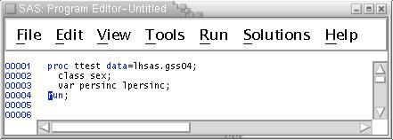
Notice that it is not necessary to retype the libname statements. They remain in force for the duration of your SAS session. Also, if you put them in a UNIX file named autoexec.sas either in your current working directory or in your home directory, it is not necessary to type them in any session.

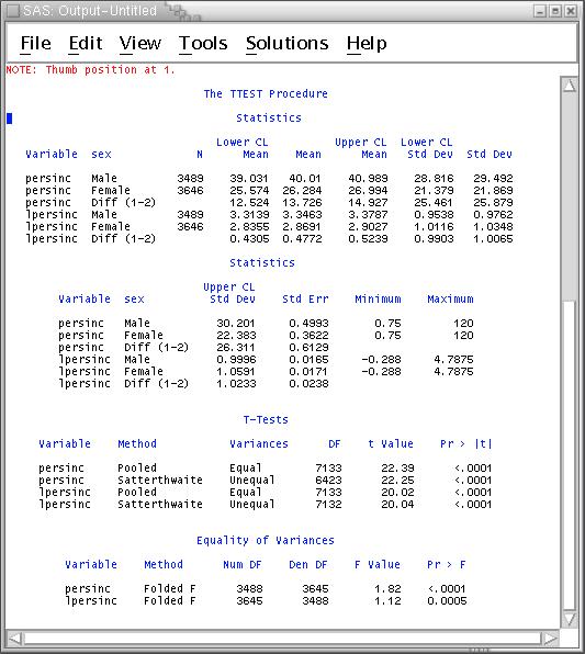
The ttest procedure produces a lot of output, considering how little it does. The top block of lines displays mean income and log income separately for women and men and the difference between the two means. It also reports confidence intervals on each mean and difference. The second block continues each line of the first block reporting additional statistics. Seeing this output, you might wish to change the linesize (ls=80) to a wider number to see if you can prevent this wrapping.

The next block reports t-tests for the difference between the mean for women and for men. The line labeled "Equal" reports tests based on the assumption that the variances (and therefore the standard deviations) for women and men are equal to each other. The line labeled "Satterthwaite" reports tests assuming these two variances are not equal. The last block of output reports tests of the equality of the variances. Use the output for the t-tests labeled "Equal" only if this block reports nonsignificant differences and the lines labeled "Satterthwaite" otherwise.

Satterthwaite is a method of calculating degrees of freedom that is more accurate than older methods.

Exercise: Race-gender differences with proc glm

Since the race variable has three categories, proc ttest is not appropriate for testing racial differences. Also, the ttest procedure permits only one independent variable in each test. Therefore, it cannot be used to test for gender differences controlling for race nor for race differences controlling for gender.

To illustrate use of the general linear model procedure (GLM), this exercise tests for both sex and race differences in income and log of income. Type the following lines into the Program Editor --

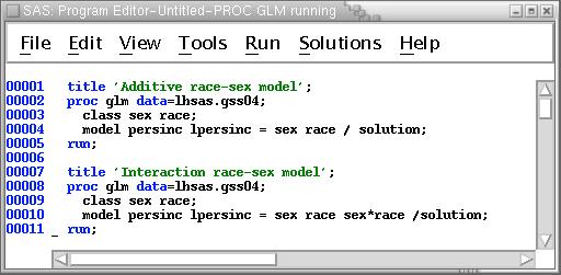
Then run the job and view the output. Note the following --

• Function of the class statement in GLM

• Limitation to only one model statement per GLM proc step
• Use of the title statements to separate the output from the two models

• Use of asterisk (*) to denote interactions in the model statement

• Use of the solution option to tell SAS to print coefficient estimates (regression coefficients)

• Message of singular X'X matrix, ignore this

• Use of dots (.) in the output to indicate the reference categories

• Reference category is the "last" category in sort order. If an explicit format is assigned, as is the case for sex and race, the default order is the formatted value. Hence, since white sorts to the last position, it is the reference racial category. In general, this is not real easy to control.

• Type I vs type III sum of squares former is hierarchical, latter is simultaneous. Use the ss3 option on the model statement to restrict the F-test to Type III, e.g.

    model persinc lpersinc = sex race sex*race / solution ss3;

Exercise: Age-Income Curve

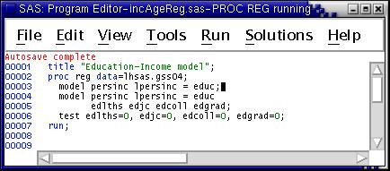
Past research shows that the relationship of age to income is not linear. The next exercise explores this nonlinearity. It uses a variable called ageSq which was created by the data-prep program which created the SAS data set. It is defined as the square of the quantity: age minus its mean..

Type the following program into the Program Editor:

This exercise shows how to use the reg procedure and the glm procedure to achieve the same result. Note the use of more than one model statement in proc reg; this constrasts with the rules for proc GLM. And note the use of the interaction notation (age*age) in the glm procedure to get the square of age without having to create it in a data step.

Run the job and check the saslog. Be sure the job ran correctly, then recall the program and save it to a file named reg_inc.sas. We will use it again later.

After the job runs correctly, view the output. There is a significant coefficient associated with the square of age in all the regressions. These results confirm past research which finds a nonlinear association between age and income. The significant t-test associated with agesq indicates that the age-income curve bends. In this case, it increases to about 50 years old and declines thereafter.

But there appears to be descrepancies between the parameter estimates produced by proc reg and proc GLM. For proc reg and persinc --

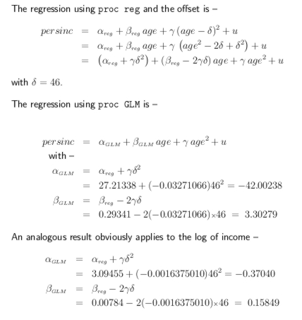
Notice that the coefficients and standard errors associated with Age² are the same for the two procedures (though proc GLM prints more digits than proc reg). Estimates of the intercept and the age "main effect" differ substantially between the two procedures, however. The reason is that the SAS variable ageSq used in the regression is defined by subtracting the constant46 before taking the square: ageSq = (age-46)**2;. But the product syntax age*agewas used in the GLM procedure, so that the square is defined without first subtracting 46.

Despite the apparent difference between the two sets of output, they are entirley consistent. They produce exactly the same predicted values, and a little elementary algebra shows that the coefficients produced by one procedure can be calculated from those produced by the other procedure.

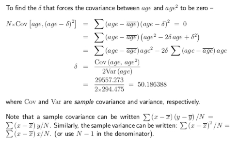
Recall that the reason for subtracting 46 from age before taking the square is to reduce the correlation between age and ageSq. The correlation between age and its square in this GSS survey is 0.98325. The correlation beteen age and ageSq is 0.41035.

A little additional elementary algebra shows that it is possible to calculate a constant that reduces this correlation exactly to zero.

Exercise: Using the where statement to exclude retired persons

We might expect that part of the strong effect of age squared is due to inclusion of retired persons in the sample. An easy way to exclude them is to use the where statement. To do this, insert a where statement in the regression procedure --

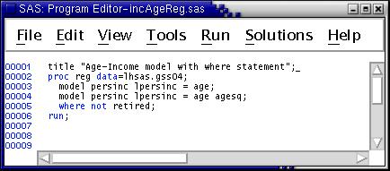
Run the job again and view the output. The results indicate that inclusion of retired persons in the sample does not affect the age-income curve very much. The reason is that most of the retired persons have missing values for income (legitimate missing due to the way the question is asked).

Exercise: Education-income relationship

There is some question about whether number of years of education, degrees earned, or both are needed to capture the relationship between income and education. The next exercise addresses these issues.

Type the following analysis program into the Program Editor. You can recall the last program and edit it if you like --

Run the job and view the output. Note the use of the test statement associated with the second model; it simultaneously tests that the effects of all the dummy variables describing degrees (edlths, edjc, edcoll, edgrad) are zero.

Also, note the omission of the degree dummy variable for high school (edhs). This means that the "reference category" consists of those whose highest degree is a high-school diploma. It is always necessary to leave out one dummy variable in a set used to describe a single categorical variable. The omitted dummy corresponds to the value of the categorical variable to be used as the reference category.

The first model is included to show how much the effect of years of schooling declines after degrees are added to the model. The findings suggest that degrees are more important than years of education. But that years of schooling remains statistically significant even after degrees are controlled.

Exercise: Proc GLM for education effects

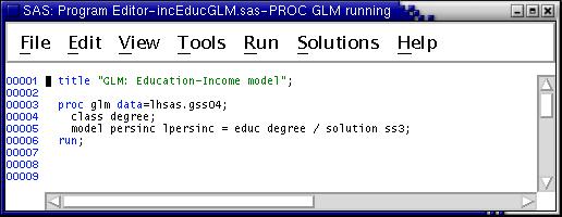
The general linear model procedure, GLM, often can be used to carry out the same analyses as done by proc reg. Advantages of GLM over the regression procedure include its ease of use with categorical variables, ease of testing for interaction, and versatility (e.g., multivariate analysis, repeated measures, testing for differences between pairs of means). Disadvantages include lengthy, cryptic output, difficulty controlling the reference category in calculating effects of categorical variables, and limitation to one model statement per GLM procedure.

To illustrate the same analysis we just did with proc reg, except this time using proc GLM, type the following commands into the Program Editor --

Note --

• Use of the class statement and the degree categorical variable in proc GLM. This substitutes for the sequence of dummy degree variables in proc reg and the test statement

• Match between the F test on degree in GLM and the F test for the test statement in reg

• R-squares, sum of squares, and F values are the same with reg and GLM

• Coefficient on the covariate (educ) is the same for reg and GLM

• Correspondences between coefficients associated with the dummy variables in proc reg and categories of degree in proc GLM.

• Trick used to force high-school diploma to be the reference group

Exercise: Several regressors

In the next exercise, we combine results from previous exploratory analyses by running regressions for log of income and income including several regressors: race and gender dummy variables, age and age squared, degree dummy variables, years of schooling, and occupational prestige. Type this program into the Program Editor

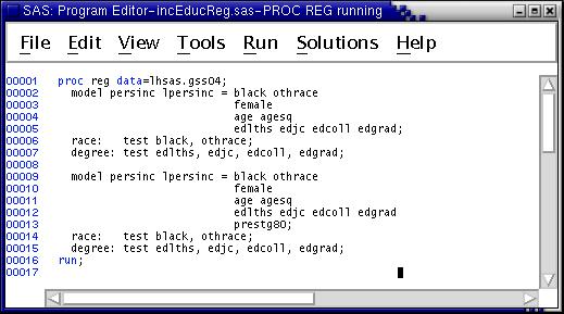
Run the job and view the output. Several points are noteworthy --

• Use of SAS free-format to separate the independent variables on different lines

• Use of labels on the test statements to identify them in the output

• The equivalence of --

     race:  test black=0, othrace=0;

  and

     race:  test black, othrace;

• Need to place test statements after each model statement

The results indicate: (1) effects of gender are not explained by education or occupational prestige differences between men and women; (2) effects of race are explained by the other variables in the model; and (3) much of the effects of education operate through occupational prestige.

Note: A model should be run using either (1) hourly wage as the dependent variable, or (2) annual hours worked as one independent variable. Some economists argue that earnings differences between women and men are mostly due to choices made by women to work fewer hours. It is possible to create a very rough estimate of annual hours with the GSS data, but it is very rough. Still, if this were a bonified research project, it should probably be done, or other data sets incorporated into the analysis.