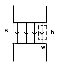
41. Apply Ampere's Law to the dashed path, to get

Integral (B ^. dA) = m₀ I_enclosed

B h = 0

B = 0

and the last equation is a contradiction, since a magnetic field is in fact present. The only assumption in this argument is the shape of the lines of B, which must therefore be drawn incorrectly.

You can cure the problem by letting the lines of B curve outward near the edge of the magnet. If done properly, the integration along the horizontal sides of the dotted path can exactly canel the integration along the vertical side inside the magnetic field.

42.

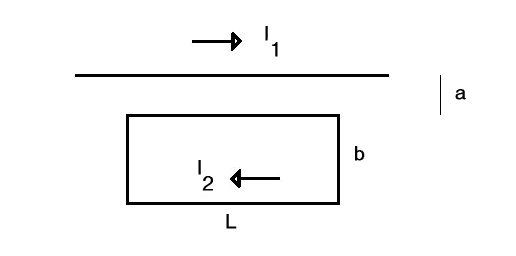
You can find the magnetic field due to I₁ by drawing a circle a distance r from the wire and applying Ampere's Law:

Integral(B^.dl) = m₀ I₁

B = m₀ I₁ / (2 p r)

The field goes into the page inside the rectangular loop. By the right-hand rule, all the forces on the loop are perpendicular to the wire pointing away from the center of the rectangle. The two forces on the wires of length are the same size but opposite in direction, so they cancel. The forces on the wire closest to I₁ and on the wire further from I₁ are, respectively:

F₁ = m₀ I₁I₂ L / (2 p a ) and

F₂ = - m₀ I₁I₂ L / [2 p (a + b) ]

taking up to be the positive direction. The sum of these two is the net force on the loop,

43. Done in class.

44.
Known

Radius of coil	R
Length of coil	L
Turns per unit length	n
Total turns	N = n L

To determine

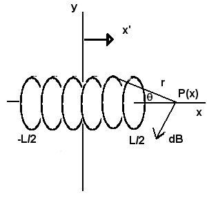
  Magnetic field B(x) at P
The y and z components of the magnetic field vanish by symmetry. The Biot-Savart law for the x component of the field in this geometry is

dB_x = - m₀ I dL sin q / (4 p r²)

We can also tell from the diagram that

r² = R² + (x - x')²

sin q = R / r

Thus q and the distance to point P is the same from any point on the loop at x'. The integral around the loop is therefore easy and gives

B_x(x) = - m₀ I R sin q / (2 r²)

         = - (1/2) m₀ I (R² / r³)

(The x-dependence is hidden in r). To sum over all the coils, we use the same trick we used last semester in getting the average "weight" of marbles falling onto a scale: multiply by the number of coils per meter and integrate over dx'. The expression is

B_x = - integral_-L/2^L/2 [n (1/2) m₀ I (R² / r³]

The integral is done by using the trigonometric substitution

x - x' = R cot q

dx' = R dq / sin² q

where q is the same angle as shown in the diagram; in other words sin q = r / R . We get

B_x = - integral_qi ^q_f [(1/2) m₀ I n sin q dq ]

which gives

where q_i and q_f are the values of q at the leftmost coil and rightmost coil, respectively. Analytically,

cos q_i = {x + L/2} / {sqrt [R² + (x + L/2)² ] }

cos q_f = {x - L/2} / {sqrt [R² + (x - L/2)² ] }

45. Use the diagram and notation of the previous problem.

Using the (previous) diagram the distances between P and the two ends of the coil are

r_i = x + L/2

r_f = x - L/2

and each r << R when P is far from the ends of the coil. Writing the magnetic field from problem 44 in terms of r_i and r_f, we get

B_x = (1/2) m₀ I n [r_f / sqrt(R² + r_f² ) - r_i / sqrt(R² + r_i² ) ].

Expanding in terms of the small ratio r_i/R we have

r_i/ sqrt(R² + r_i²) = (r_i / R) / sqrt(1 + r_i² / R² ) = 1 - R² / (2 r_i² )

and a similar expression involving r_f . These two expressions can be substituted into the expression for B to give

which is the result we were supposed to get.