Distributions

1. CLASS 9 AGENDA:
1. Populations and samples
2. Distributions
3. Percentiles and Quartiles
4. The summation sign
5. Reading:
1. Agresti and Finlay, Statistical Methods for the Social Sciences, chapter 3.



2. POPULATIONS AND SAMPLES:
1. Population: a well-defined collection of units of analysis such as the American states, the people living in Delaware, the countries in Asia, the students taking this course.
2. Sample: a subset of the population drawn in some fashion. We can have, for example, a sample of the states, a sample of Delawareans, or a sample of students taking this class.
3. Simple Random Sample (SRS): a sample drawn from the population in such a way that each member has an equal chance of being included.
4. Sample size, N.
1. Size of the sample greatly affects precision or reliability of estimators (see below) but not validity as usually defined.
5. Parameter: a statistical characteristic (e.g., mean, standard deviation) of a population. Two major goals of statistics are to estimate population parameters and to test hypotheses about them.
1. Parameters are usually denoted with Greek letters.
1. Example: the mean, usually denoted by , is a parameter.
2. Order statistics, however, are denoted with capital letters as in M for median and H_l and H_u for lower and upper hinges respectively.
6. Sample statistic: a characteristic of a sample or batch of values that is generally used to make inferences about the corresponding population parameter. (Often called an estimator.)
1. Sample statistics are frequently denoted by a Greek letter with a hat over it (e.g., ) but not always as in the case of the sample mean, .



3. DISTRIBUTIONS:
1. One purpose of explaining distributions at this point is lay a foundation for the discussion of statistical inference. Statistical inference involves, among other things, hypothesis testing. A statistical hypothesis, loosely speaking, is a statement about a population parameter or set of parameters. For example, we might hypothesize that a population mean () has a particular value or that two sub-population means (₁ and ₂) do not differ. A hypothesis is tested by applying statistical theory to a sample result. Statistical theory, in turn, depends on probability or theoretical distributions.
2. But we also need to take into account the shape of empirical (or observed) distributions because
1. they affect our interpretation of numbers
2. we may have to transform the original data in order to draw correct inferences from them.



4. SHAPES AND TYPES OF DISTRIBUTIONS:
1. Observed Frequency Distribution: the number (frequency) of cases at each value or range of values of a variable.
1. Example: all the stem-and-leaf displays we have drawn are examples.
2. Frequency distributions show how many observations have various values of the variable.
3. One can thus determine how many cases will be above or below a given point.
2. Shapes and properties of empirical distributions
1. Note: these are "ideal" types. Observed distributions will only approximate these shapes.
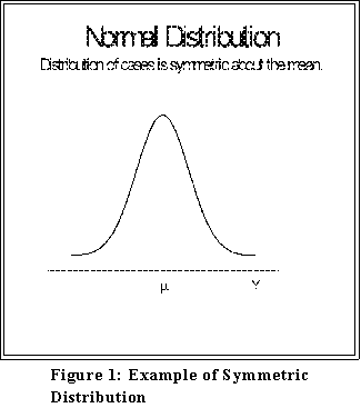
2. Symmetric distributions: proportion or number of cases on either side of the mean is roughly equal.
3. A "normal" or bell-shaped distribution is the perfect example of a symmetric distribution.

1. Although we will look at the normal distribution more closely next week, for now notice that it has the properties, which incidentally further clarify the meaning of the standard deviation. (See Agresti and Finlay, Statistical Methods, page 60.
1. About two thirds (approximately 68%) of the data fall within plus and minus one standard deviation of the mean.
2. About 95 percent fall between plus and minus two standard deviations of the mean.
3. About 99 percent lie within plus or minus three standard deviations of the mean.
2. Many observed data sets with a reasonable number of cases (N > 50) have so-called normal distributions.
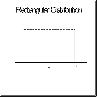
3. Another symmetric distribution is called rectangular.

1. Since the cases or observations are spread evenly on both sides of the mean, the distribution is symmetric.
2. It shape can be observed from a stem-and-leaf display.
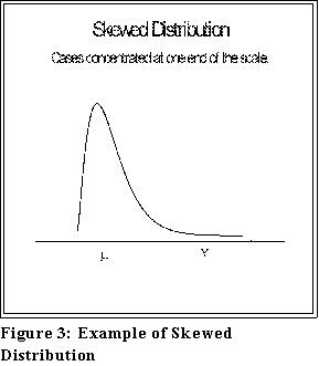
1. Skewed distributions. Figure 3 provides an example.

1. A distribution may be skewed to the left, as here, or to the right.
2. Data that are skewed in this manner are frequently transformed in such a manner that the skewness is more or less removed before being further analyzed.
3. As we have noted before, the mean and median will usually differ considerably in these situations.
1. Probability distributions: very loosely speaking, a probability distribution tells for each measurement interval or class the probability of its occurrence.
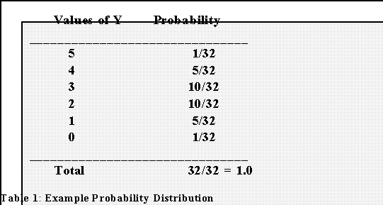
1. Example: consider an "experiment" consisting of 5 tosses of a "fair" coin (i.e., the probability of heads is one-half). The probability distribution for this experiment gives the probability of obtaining Y number of heads. (Y--the number of heads in five tosses--is the variable; the distribution indicates the probability of obtaining each value of Y.)

1. Uses:
1. We can relate a particular sample result to its probability of occurrence under some hypothesis or condition. We know, for example, that if a coin is "fair" the probability of getting one head in 5 tosses is 5/32.
1. You can arrive at this number by sheer reasoning but looking at the above probability distribution makes the task very easy.
2. We can relate a range of outcomes to their probabilities. The chances of getting 1 or fewer heads in 5 tosses is thus 5/32 plus 1/32 or 6/32.
3. In general, a probability distribution helps one test hypotheses about a population.
1. Probability distributions are described by parameters, usually the mean and standard deviation (sometimes called a standard error), and shape or form of the graph that describes them.



1. PERCENTILES AND QUARTILES:
1. A more general notion of order statistic than the median or hinge is the percentile, which Agresti and Finlay (page 52) define as a number such that a certain percent of the observations fall below it.
2. More precisely, the p^th percentile is the number, Y_p, such that p percent of the cases fall below it and (100 - p) are above it.
3. Examples: for a particular distribution or batch of data the 50^th percentile, the median, is the number such that 50 percent of the observations lie above and 50 percent below it.
4. The 90^th percentile is the number that divides the distribution such that 90 percent of the cases are above it and 10 percent below.
5. Two commonly used percentiles are the upper and lower quartile.
1. The lower is usually called the 25^th percentile because 25 percent of the cases lie below it; and the upper is termed the 75^th percentile since 75 percent of the cases are below it.
2. Example
3. Most statistical programs report quartiles along with the median and mean.
4. Moreover, as Agresti and Finlay note (page 23), box plots are sometimes constructed to show the quartiles. In fact, this is the default for MINITAB.
5. The difference between the upper and lower quartiles is called the interquartile range.
6. Examples:
1. The data section of the course web page contains a file called "Pennsylvania County Data."
1. There are 67 counties (units of analysis)
2. The variables are:
1. County identification code. Not of any great use now.
2. Percent of all persons in the county who are poor.
3. Percent of children 5 to 17 who are poor
4. Median household income.
2. Here are some statistics for percent of persons in the county who are poor.
1. Median: 12.3%
2. Lower quartile (Q1): 9.1%
3. Upper quartile (Q3): 14.5%
4. Interquartile range: 5.4%
5. Lower hinge: 9.6%
6. Upper hinge: 14.45%
1. Note that because of the way hinges and percentiles are defined they are not quite the same. But in most cases they are functionally equivalent.



2. SUMMATION SIGN OPERATIONS:
1. The summation sign, capital sigma, simply means addition. Assume that we have N cases or values of a variable, Y.

1. This the sum of Y.
1. The symbol directs us to add the Y's starting with the first and ending with the Nth. So far, no problem.
2. Rules and elaborations:

1. This is the sum of the Y's squared
1. Note:

1. Example: data 12, 3, 9, 17, 51

1. whereas

1. If a is a constant, then

1. Example, using previous data and let a = 2

1. Sum of the product of two variables, Y and X:

1. Suppose X and Y are variables:

				Y		 X
				 _________________
				12		 3
				 3		 1
				 9		-2		
				17		 4
				51		-1

1. Then

1. This total is called the sum of cross products



1. NEXT TIME:
1. Histograms
2. Odds ratios and other summary statistics and methods
3. The normal distribution.

Go to Statistics main page

Go to H. T. Reynolds page.

Copyright © 1997 H. T. Reynolds