lab07, CISC105, Fall 2007

Overview

In this lab, we'll cover some basic things about MATLAB, and get more practice with matrices, function M-files, and test scripts.

Step-by-Step Instructions

Step 1: Preliminaries

To prepare for this week's lab, do all the following steps. If you are not sure what to do at any stage, you can consult earlier labs for details:

Create a new directory called ~/cisc105/lab07
Copy all the files from /www/htdocs/CIS/105/haggerty/07F/labs/lab07 into your new directory ~/cisc105/lab07

Step 2: Learning a few things about MATLAB

Each of the steps under this section involves learning something interesting about MATLAB.

(Acknowledgement: The items in Step 2 of this lab (except for step 2e) are adapted from labs written by Dr. Terry Harvey, by permission.)

Step 2a: A surprise

If you type the expression0.3 - 0.2 - 0.1 at the MATLAB prompt, what would you expect the result to be?

Try it and see what result you get. Are you surprised?

Next, use the fprintf() function to examine each of the numbers involved, by changing the width and precision fields of the format specifier so that you can see the numbers with great precision

Hints: type "help fprintf" at the MATLAB prompt, do a web search on "MATLAB fprintf", and/or consult section 7.2 in your textbook.

Once you have learned how to use fprintf to do this, start a diary file called lab07_step2a.txt. In this file, show high precision versions of all the tenths from 0.1 to 1.0. Each should print on a separate line.

To turn in from this step: diary file lab07_step2a.txt

Step 2b: Growing a Matrix

We can change the size of a matrix we are using in Matlab. Start a diary file called lab07_step2b.txt.

Then, show the following sequence of commands:

x = []
x(2) = 9
x(2,2) = 8

What is the size of x after each command? Use the size function to show this (e.g. type size(x))

Being able to “grow” a matrix to fit our needs is a powerful tool, but not without cost—we pay a performance penalty when we grow a Matrix a little bit at a time.

To turn in from this step: diary file lab07_step2b.txt

Step 2c: for loop over the length of a vector

We can use the length() function on a vector to see how long it is, then use the length found to run a for loop that looks at each position in the vector.

For an example, see lengthVector.m in the files you copied for this week's lab.

You can also type help length at the MATLAB prompt to learn more about the length function.

Here's another example of a function M-file that does uses this technique.myMax.m finds the maximum value in a vector. It is in your directory this week, along with a test script called testMyMax.m, and a helper function performEqualTest.m

Note that MATLAB has a built-in function called max() that does this, but that's not the point—finding a maximum is a basic programming skill, so we need to know how to do it even without a built-in function to help us. So, read through this code carefully, because a question about it could show up on a future quiz or exam.

Notice how we initialize theMax to the first value in the vector. We then compare it to every remaining value, and in each case, if that value is bigger, we set theMax to that value instead. In this way, myMax never gets smaller, but it may get larger, and is always guaranteed to be the largest number we've seen so far. (A question to ponder: how would you modify this function M-file to return the minimum instead of the maximum?)

function theMax = myMax(v)
% myMax   return maximum value in a vector
%
% consumes: v, a vector
% produces: theMax, a scalar, the maximum value in v
%
% Example:
%   >> myMax([3 5 6 2])
%   ans =
%       6
%   >> myMax([])
%   ans = 
%       []
%
% P. Conrad for CISC105, sect 99, 10/22/2007
  
  if (length(v) == 0)
    theMax = [];
  else
    theMax = v(1);
    
    for i=2:length(v)
      
      if (v(i) > theMax)
	     theMax = v(i);
      end; % if
      
    end; % for
  end % if 

    

 return;

  
end % function

Now, for credit: Write a function M-file sevens2pi.m that traverses a vector of any length with a for loop and changes the sevens in the vector to pi. Write a simple test script testSevens2pi.m that shows your function working on both row and column vectors.

Create a diary file lab07_step2c.txt in which you type out the source code of both sevens2pi.m and testSevens2pi.m, and then show that the function passes its tests.

To turn in from this step: diary file lab07_step2c.txt, M-files sevens2pi.m and testSevens2pi.m

Step 2d: for loop over values in a vector

A function that traverses a vector does not always need to calculate the length of a vector. An example file, yetAnotherMax.m is listed below —it is yet another function that returns the maximum value in a vector. The code for that, along with a test script testYetAnotherMax.m is in your directory this week.

Note that the line of code for e = v indicates that e should take on each value of v one at a time. The for loop is repeated for each value of v. (In some programming languages, this is called a foreach loop).

We use e rather than i to indicate that we are processing elements rather than indexes (or indices, if you prefer the more proper form of the plural).

function theMax = yetAnotherMax(v)
% yetAnotherMax   return maximum value in a vector (a different way)
%
% consumes: v, a vector
% produces: theMax, a scalar, the maximum value in v
%
% Example:
%   >> myMax([3 5 6 2])
%   ans =
%       6
%   >> myMax([])
%   ans = 
%       []
%
% P. Conrad for CISC105, sect 99, 10/22/2007
  
  if (isempty(v))
    theMax = [];
  else
    theMax = v(1);
    
    for e=v % e takes on the value of each successive element
      if (e > theMax)
	theMax = e;
      end; % if
      
    end; % for
 end % if 
     
 return;
   
end % function

For credit: Write a function M-file squareVector.m that uses a for loop to compute the square of each member of its vector parameter and store the value in an output vector—but, do not (in any way) find the length of the vector parameter before using it.

Write a simple test script testSquareVector.m that shows your function working on row vectors.

Hint: also review step2b above about growing a matrix. You may need to use an extra variable.

Create a diary file lab07_step2d.txt in which you type out the source code of both squareVector.m and testSquareVector.m, and then show that the function passes its tests.

To turn in from this step: diary file lab07_step2d.txt, M-files squareVector.m and testSquareVector.

Step 2e: fixing the performEqualTest.m script

The performEqualTest.m script has a limitation—it does not behave correctly when passed empty matrices.

It should print "passed" when either

both actual and expected are empty, or
both actual and expected are not empty, and they are equal to each other

Otherwise it should print "failed".

Change the script so that it works properly.

To test it, you can:

uncomment the line % performEqualTest( myMax([]),[],'4'); in testMyMax.m
uncomment the line % performEqualTest( yetAnotherMax([]),[],'4'); in testYetAnotherMax.m
then, re-run these test scripts

Make a diary file lab07_step2e.txt in which you type out the performEqualTest.m file, and then show that it is working on these two test scripts, with test 4 uncommented.

To turn in:

revised version of performEqualTest.m, testMyMax.m, testYetAnotherMax.m
- Note: these are files that are already included in your submission from earlier steps—you don't have to submit more than one copy. The modified copy is fine for both steps.
diary file lab07_step2e.txt

Step 3: Plotting Line Drawings with MATLAB

There is nothing to turn in from Step 3—it is background for the exercises in Steps 4 and 5, and also for lab09.

Step 3a: Introduction

Suppose we have a set of points that we want to plot that represent a simple drawing---sort of a "connect the dots" style drawing.

For example, suppose we connect:

(0,0) to (2,8) to (4,0) with one line
then (1,4) to (3,4) with another line

Then the result is the capital letter A:

We can represent a drawing like this using a MATLAB 2xn matrix, as follows:

each of the n columns represents one point
the first number in each column represents a x coordinate
the second number in each column represents a y coordinate

Furthermore, we can state that if a column is an exact repeat of the previous row, this is a signal that the user should "pick up the pen" and start a new line with the next column.

With these rules in mind, we can represent out letter A as follows:

>> points = [ 0 0 ; 2 8 ; 4 0 ; 4 0 ; 1 4 ; 3 4 ]'                   

points =

     0     2     4     4     1     3
     0     8     0     0     4     4

>>

Step 3b: Plotting a drawing

How can we plot a drawing represented in this way?

The following MATLAB function M-file can do the job:

plotLineDrawing.m

For example:

>>  points = [ 0 0 ; 2 8 ; 4 0 ; 4 0 ; 1 4; 3 4 ]';
>>  plotLineDrawing(points,'-djpeg','cisc105/10.18','letterA.jpg') 

ans =

http://copland.udel.edu/~haggerty/cisc105/10.18/letterA.jpg

>>

The resulting plot looks like this:

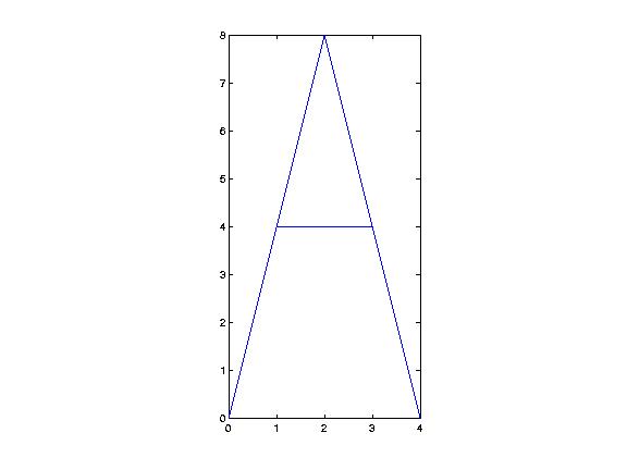
Here is another example: a very simple looking tree:


>> tree = [ 0 4 1; 5 16 1; 10 4 1; 0 4 1; 0 4 1; 4 4 1; 4 0 1; 6 0 1; 6 4 1]'

tree =

     0     5    10     0     0     4     4     6     6
     4    16     4     4     4     4     0     0     4
     1     1     1     1     1     1     1     1     1

>>  plotLineDrawing(tree,'-djpeg','cisc105/10.18','tree.jpg')                   

ans =

http://copland.udel.edu/~haggerty/cisc105/10.18/tree.jpg

>>

And here is what it looks like:

To understand the four parameters, we can use the help that is built into the H1 comment:

>> help plotLineDrawing
 plotLineDrawing   plot points as a line drawing on the web
 
  consumes: 
    points, a matrix of points to plot 
                    each column is one point (x,y)
                    the first row is all the x values
                    the second row is all the y values
 
                    if there are more then 2 rows, the rest of the
                    rows are ignored; if fewer, an empty matrix is returned
 
                    if a column is repeated, it means pick up the pen
 
    graphicsType: one of the following '-djpeg', '-dpng'
                  (or other legal arg to the function print())
 
    dirName: directory name, relative to ~/public_html
    fileName: a filename in which to store the drawing
 
  produces:
    url: the url at which the graphic can be found, or
         an empty matrix if the graphic cannot be produced.
   
  Example: Plot the capital letter A in the box with 0,0 at lower
           left and 4,8 at upper right.
 
   >> points = [ 0 0 ; 2 8 ; 4 0 ; 4 0 ; 1 4; 3 4 ]';
   >> plotLineDrawing(points,'-djpeg','cisc105/10.18','letterA.jpg') 
   ans = 
 
     http://copland.udel.edu/~haggerty/cisc105/10.18/letterA.jpg
 
   >> 
  P. Conrad   for CISC105, 10/16/2007

>>

Step 3c: Affine transformations

Once we have these points in this fashion, we can apply what are called the Affine Transformations:

These are the transformation that translate, rotate, and scale.

Translate means to "shift the coordinate system by tx in the x direction, and ty in the y direction." It is how we move a figure.

Rotate means to "rotate the entire coordinate system around the origin by some angle phi". It is how we rotate figures.

Scale means to "stretch the coordinate system by a factor of sx in the x direction and sy in the y direction." It is how we make a figure bigger or smaller.

To use these transformations, we have to add an extra row of 1's to our points. So instead of:

>> points = [ 0 0 ; 2 8 ; 4 0 ; 4 0 ; 1 4 ; 3 4 ]'                   

points =

     0     2     4     4     1     3
     0     8     0     0     4     4


>>

We have:

>> points = [ 0 0 1; 2 8 1; 4 0 1; 4 0 1; 1 4 1; 3 4 1]'                   

points =

     0     2     4     4     1     3
     0     8     0     0     4     4
     1     1     1     1     1     1
>>

Fortunately, our plotting routine doesn't care if this extra row is there---it just ignores it.

Why this extra row of ones? The short answer is: it makes the math work out. For a more satisfying answer, take a linear algebra course, a computer graphics or do some research on the web or at the library. For our purposes, we'll take this as given.

With this extra row in place, we can do scaling very easily. For example, if we want to scale the letter A by a factor of 3 in the x direction, and a factor of 4 in the y direction, we can type this:

>>  points = [ 0 0 1; 2 8 1; 4 0 1; 4 0 1; 1 4 1; 3 4 1]'          

points =

     0     2     4     4     1     3
     0     8     0     0     4     4
     1     1     1     1     1     1

>> s = scaleIt(3,4)

s =

     3     0     0
     0     4     0
     0     0     1

>> newPoints = s * points 

newPoints =

     0     6    12    12     3     9
     0    32     0     0    16    16
     1     1     1     1     1     1

>>  plotLineDrawing(newPoints,'-djpeg','cisc105/10.18','scaledA.jpg') 

ans =

http://copland.udel.edu/~haggerty/cisc105/10.18/scaledA.jpg

>>

And the resulting plot looks like this:

The .m file for the scaleIt() function, scaleIt.m is very simple--with the exception of the H1 comment, it is really little more than one line of code:

function result = scaleIt(sx,sy)
% scaleIt   return matrix for scaling of 2D graphics

...

  result = [ sx 0 0; 0 sy 0; 0 0 1];
  return;
end

Here's a link to the complete code: scaleIt.m

Step 4: Write the functions for translating and rotating

Using the scaleIt.m function M-file given above as an example, and the affine formulas given earlier on this web page for translation and rotation, write similar function M-files to produce functions like these:

(a) a function to do translation

function result = translateIt(tx,ty)
%rotateIt   matrix for 2D translation by tx and ty

(b) a function to do rotation

function result = rotateIt(phi)
%rotateIt   matrix for 2D rotation around origin by phi radians

(c) as a convenience, a function that rotates in degrees instead of radians:
(hint: use a call to the radians version inside your function body).

function result = rotateItDeg(phi)
%rotateIt   matrix for 2D rotation around origin by phi degrees

In each case, write the function M-file, and a test script.

Then:

Write a script M-file called initPlot.m that will plot your three initials into a file called init.jpg inside the directory ~/public_html/cisc105/lab07/step4, by calling plotLineDrawing with appropriate parameters.
Once that is working, add lines into initPlot.m that also create three more plots, demonstrating that you can translate, rotate, and scale your initials. Call the files translate.jpg, rotate.jpg, and scale.jpg

Finally

Make a diary file lab07_step4.txt in which you demonstrate that the functions work.

To turn in:

M files: translateIt.m, testTranslateIt.m, rotateIt.m, testRotateIt.m, rotateItDec.m, testRotateItDeg.m
Diary file: lab07_step4.txt

On the web

Step 5: Fixing the axes

Some figures---for example, a square---don't look too good with the axis equal tight command that is inside plotLineDrawing.m. For example, while we can plot the letter A just fine, if we plot the letter L, we'll see nothing, because the lines are coincident with the x and y axes.

Similar, if we plot a square, all four edges will be obscured by the edges of the plot.

To fix this, you can write a function findLimits like this:

function [xmin xmax ymin ymax] = findLimits(points)
%findLimits  find x,y limits in a set of points for a line drawing
%
% consumes: points, a matrix of points (in format expected by plotLineDrawing.m)
%           see "help plotLineDrawing" for more details
%
% produces: xmin, xmax: the minimum and maximum values from points(1,:),
%                        i.e. the x coordinates of all the points in the drawing
%           ymin, ymax: the minimum and maximum values from points (2,:),
%                        i.e. the y coordinates of all the points in the drawing
...

Then, make a new version of plotLineDrawing.m that uses this function like this:

   [xmin xmax ymin ymax] = findLimits(points);
   axis ([xmin-1  xmax+1  ymin-1  ymax+1]);

Another option is to write the function as:

function limits = findLimits(points)

and have the function return a vector containing the four elements. In that case, you'll have to do a bit more work inside the plotLineDrawing() function to adjust the four values before passing them to the built-in axis function of MATLAB.

You should also figure out how you can also specify that you want the "equal" option on the axis command so that the aspect ratio is preserved---that is, the x and y units are the same size on the plot that is produced.

What you need to do for credit

Write a test script M-file testFindLimits.m, following the example of test scripts from earlier labs,
Write the function M-file findLimits.m
- first in stub form (i.e. returning a stub answer such as [-42 42 -42 42] for all inputs, in order to "test the test script" (all tests should fail)
- then in a form that will actually work (all tests should pass)
Then, put a function call to findLimits() into plotLineDrawing.m so that when you plot a drawing, the axes will be set so that there is one unit of space around the drawing.
To test this file, re-run the initPlot.m from step 4, and see if the plots now have space around them.
No diary is necessary for this step.

To do this properly

First, write a test script, called testFindLimits.m,
Then, write a stub version of the findLimits.m function M-file (it can always return [-42 42 -42 42]) to make sure that the test script works (i.e. all the tests fail)
Then, change findLimits.m so that it passes all the tests
Finally, put the code into plotLineDrawing.m , and try running initPlot.m and looking at the plots.

Here are a few. test cases to help you in your thinking. Let's suppose that you are using this as your prototype (though it is your choice whether to use this, or the [xmin xmax ymin ymax] version)

function limits = findLimits(points)

If the input is the A matrix shown below:

>> A                

A =

     0     2     4     4     1     3
     0     8     0     0     4     4
     1     1     1     1     1     1

>> actual = findLimits(A)
...

then the expected value would be [0 4 0 8].

But if the input were the house matrix:

>> load house.dat
>> house

house =

    40   120   120    40    40    40    40    80   120   120    72    72    88    88
    80    80   170   170    80    80   170   200   170   170    80   125   125    80
     1     1     1     1     1     1     1     1     1     1     1     1     1     1

>> actual = findLimits(house)
...

In this case, expected should be [40 120 80 200]

If you have any questions about exactly what you are supposed to do, ask your instructor or your TA.

Um, I'm stuck---I know what I'm supposed to do, but I don't know how

Ok, so it turns out that MATLAB already has a function built in function called min that will help you find the smallest element in a Matrix. However, it requires you to read the documentation, which can be found here:

http://www.mathworks.com/access/helpdesk/help/techdoc/index.html?/access/helpdesk/help/techdoc/ref/min.html

You have to figure out exactly how to get at what we want, which is:

the smallest x coordinate
the largest x coordinate
the smallest y coordinate
the largest y coordinate

Some questions to guide you:

How do we select out just the first row of the points array, and return it as a row vector?
How do we select out just the second row of the points array, and return it as a row vector?
If you pass a 2-dimensional array into min, what does it return?
Would it help to transpose the points array (i.e. to use points' instead of points?
If the link above is a link to the documentation for the min function, how do you think you could find the documentation for the max function?

Some additional suggestions:

Try coming up with various arrays, and passing them into the MATLAB min and max functions and see what you get.
If you can get the answers into four scalar variables called xmin, xmax, ymin and ymax, then you can just set result=[xmin xmax ymin ymax] to construct the result matrix that you are supposed to return.
So, as a first step, concentrate on coming up with just one of the four numbers. If you can get just one of the four numbers, you can use similar steps to come up with the other three.

Step 6: Make a zip file lab07.zip of your files

As with last week, we are going to create a zip file. This time we are just going to take all .m, .txt and .dat files inside your lab07 directory. The diary files will be included inside your zip file, so that's the only file you'll have to submit on WebCT.

To create and test the zip file, follow the instructions from step11 of lab06 and/or lab07.

Step 7: Submit your lab07.zip file

Now you can submit your work on WebCT, and you are done!

Grading: 100 Points

step	what we're looking for	points
step 2a	`lab07_step2a.txt`10 pts for following directions (i.e. showing value of 0.1, 0.2, etc. at high precision)	10
step 2b	`lab07_step2b.txt` 10 pts for following directions (i.e. showing size of matrix after each step)	10
step 2c	`sevens2pi.m` (5 pts for correctness, 5 for style) `testSevens2pi.m` (5 pts for correctness, 5 for style) `lab07_step2c.txt` (10 pts)	30
step 2d	`squareVector.m` (5 pts for correctness, 5 for style) `testSquareVector.m` (5 pts for correctness, 5 for style) `lab07_step2d.txt`(10 pts)	30
step 2e	`performEqualTest.m` (5 pts for correctness of changed file, 5 for style) `lab07_step3e.txt` (10 pts)	20
step 4	M-files: 10 pts each (5 for correctness, 5 for style)`,` 60 pts total`translateIt.m, testTranslateIt.m, rotateIt.m, testRotateIt.m, rotateItDec.m, testRotateItDeg.m` Diary file: `lab07_step4.txt` (10 pts) On the web: (10 pts each, 40 pts total) `http://copland.udel.edu/~youruserid/cisc105/lab07/step4/init.jpg` `http://copland.udel.edu/~youruserid/cisc105/lab07/step4/translate.jpg` `http://copland.udel.edu/~youruserid/cisc105/lab07/step4/rotate.jpg` `http://copland.udel.edu/~youruserid/cisc105/lab07/step4/scale.jpg`	110
step 5	`testFindLimits.m` (5 pts for correctness of changed file, 5 for style) `findLimits.m` (5 pts for correctness of changed file, 5 for style) function call to `findLimits()` in `plotLineDrawing.m` (5 pts) fixing the aspect ratio with correct use of `equal` option of `axis` built-in function (5 pts) re-running initPlot.m, as reflected in the fact that plots on the web from step 4 have the extra space around them. (20 pts, 5 pts each) No diary is necessary for this step.	50
step 6	Correctly creating the lab07.zip file	20
step 7	Submitting only lab07.zip on WebCT	10
overall following of directions	student should follow any and all other directions given	10
Total