Lab04, CISC105, Fall 2007

Overview

This week, in lab04, you will learn how to start with a simple data file of numbers—in this case, data about Hurricane Katrina (from August of 2005)—and end up with two graphs

• a map showing the path of Hurricane Katrina (longitude on the x axis, and latitude on the y axis)
• a graph showing the relationship between air pressure and wind speed

In the process, you'll also learn a few things about slicing up Matrices in MATLAB, i.e. selecting out particular rows and columns.

In a future lab, we'll add two more graphs:

• a graph showing the relationship between elapsed time from the start of the storm, and wind speed
• a graph showing the relationship between elapsed time from the start of the storm, and air pressure

And we'll also learn how to incorporate all four graphs into a simple web page.

Goals

By the time you complete this lab, you should be able to:

1. Work with the "load" command to load in some numerical data from an ASCII formatted data file.
2. Be able to select out a "column" from a matrix
3. Plot two column vectors on the x and y axis, and put a legend and title on your graph
4. Save the results of your plots to a graphic file suitable for use on the web.

You will also get more practice with

1. Managing directories in MATLAB with the pwd, mkdir, and cd commands.
2. Converting simple mathematical formulas into MATLAB assignment statements
3. Saving a sequence of MATLAB commands into a script M-file

By now we assume you are entirely familiar with these items, and will no longer describe them in detail:

1. Creating a new subdirectory (such as ~/cisc105/lab04)
2. Copying files from a directory on strauss into your current directory
3. Submitting your saved work for grading using "MyCourses" (also known as WebCT).

Since this lab involves plotting...

There are advantages to using a SunRay...

On a SunRay, you can see the results of a plot instantly in a separate graphics window.

... but you can still do the lab on any machine with SSH access to strauss

If you do the lab on a PC or Mac, there are some extra steps involved—you have to first create the plot, then save it to a graphics file (a .jpg file), then make it readable on the web, and finally look at it in a web browser.

However, we can use script and function M-files to partially automate this process, making it much less burdensome.

Step-by-Step Instructions

Step 1: Preliminaries

To prepare for this week's lab, do all the following steps. If you are not sure what to do at any stage, you can consult earlier labs for details:

• Create a new directory called ~/cisc105/lab04
• Copy all the files from /www/htdocs/CIS/105/haggerty/07F/labs/lab04 into your new directory ~/cisc105/lab04

Step 2: Loading the file katrina.dat into a MATLAB matrix called katrina

Step 2a: Becoming familiar with the file katrina.dat

In step 1, you copied files called katrina.txt, katrina.dat and lab04a.m into your ~/cisc105/lab04 directory.

• The file katrina.txt is a text file that explains the numbers inside katrina.dat.
• Example the contents of katrina.dat with one of the following commands:
  • Use the Unix command more katrina.txt
  • Or, use the MATLAB command type katrina.txt
• The file katrina.dat is an example of an "ASCII formatted data file."
  • ASCII formatted means you can type out the contents with regular Unix commands, and you can edit the contents with editors such as emacs or vi on Unix, TextEdit on the Mac, or Notepad on Windows.
• Examine the contents of katrina.dat with one of the following commands. You'll just see a bunch of numbers.
  • Use the Unix command more katrina.dat
  • Or, use the MATLAB command type katrina.dat
• The lab04a.m file is a partially complete example of a script M-file that will plot data from katrina.dat and put the resulting graph on the web. We'll work with this file in Step 3b of this lab.

Step 2b: Loading katrina.dat into MATLAB

We are going to use the command load katrina.dat to load the contents of that file into a MATLAB matrix called katrina. Start up MATLAB from the directory ~/cisc105/lab04 (or cd into ~/cisc105/lab04 after you are in MATLAB) and try the following commands—hopefully your results are as shown below.

>> load katrina.dat
>> katrina

katrina =

   1.0e+03 *

    0.0180    0.0230    0.0231    0.0751    0.0350    1.0080
         0    0.0240    0.0234    0.0757    0.0350    1.0070
    0.0060    0.0240    0.0238    0.0762    0.0350    1.0070
    0.0120    0.0240    0.0245    0.0765    0.0400    1.0060
    0.0180    0.0240    0.0254    0.0769    0.0450    1.0030
         0    0.0250    0.0260    0.0777    0.0500    1.0000
    0.0060    0.0250    0.0261    0.0784    0.0600    0.9970
    0.0120    0.0250    0.0262    0.0790    0.0650    0.9940
    0.0180    0.0250    0.0262    0.0796    0.0700    0.9880
         0    0.0260    0.0259    0.0803    0.0800    0.9830
    0.0060    0.0260    0.0254    0.0813    0.0750    0.9870
    0.0120    0.0260    0.0251    0.0820    0.0850    0.9790
    0.0180    0.0260    0.0249    0.0826    0.1000    0.9680
         0    0.0270    0.0246    0.0833    0.1050    0.9590
    0.0060    0.0270    0.0244    0.0840    0.1100    0.9500
    0.0120    0.0270    0.0244    0.0847    0.1150    0.9420
    0.0180    0.0270    0.0245    0.0853    0.1150    0.9480
         0    0.0280    0.0248    0.0859    0.1150    0.9410
    0.0060    0.0280    0.0252    0.0867    0.1450    0.9300
    0.0120    0.0280    0.0257    0.0877    0.1650    0.9090
    0.0180    0.0280    0.0263    0.0886    0.1750    0.9020
         0    0.0290    0.0272    0.0892    0.1600    0.9050
    0.0060    0.0290    0.0282    0.0896    0.1450    0.9130
    0.0120    0.0290    0.0295    0.0896    0.1250    0.9230
    0.0180    0.0290    0.0311    0.0896    0.0900    0.9480
         0    0.0300    0.0326    0.0891    0.0600    0.9610
    0.0060    0.0300    0.0341    0.0886    0.0450    0.9780
    0.0120    0.0300    0.0356    0.0880    0.0350    0.9850
    0.0180    0.0300    0.0370    0.0870    0.0350    0.9900
         0    0.0310    0.0386    0.0853    0.0350    0.9940
    0.0060    0.0310    0.0401    0.0829    0.0300    0.9960

>> 

Compare the first three lines of output in the window above, namely:

>> load katrina.dat
>> katrina

katrina =

   1.0e+03 *

    0.0180    0.0230    0.0231    0.0751    0.0350    1.0080
         0    0.0240    0.0234    0.0757    0.0350    1.0070
    0.0060    0.0240    0.0238    0.0762    0.0350    1.0070
...

with the actual contents of the first three lines of katrina.dat, which are:

18  23  23.1   75.1      35    1008     
 0  24  23.4   75.7      35    1007     
 6  24  23.8   76.2      35    1007     

...

MATLAB has the correct matrix, but it is in a rather odd format—specifically, all the values have to be scaled by 1.0e+03 (i.e. 1.0x10³) to get the true value. That's the meaning of the the first part of the MATLAB output for the matrix called katrina, namely the 1.0e+03 * on the first line of the output for the matrix katrina.

We can tell MATLAB to give us the numbers in a nicer format with the command format short g, as shown below. Read about the format short g command (and other related commands) on pages 40 and 41 of your text (section 2.6), and try the command out below. You might also try some of the other commands on p. 41, to see what the matrix looks like with those formats.

>> format short g
>> katrina

katrina =

           18           23         23.1         75.1           35         1008
            0           24         23.4         75.7           35         1007
            6           24         23.8         76.2           35         1007

etc... some lines omitted here

          
            6           31         40.1         82.9           30          996

>> 

Step 3: Plotting the data from the Matrix katrina as a map of longitude and latitude

Now that we have the data into MATLAB, we can do some interesting plots.

Step 3a: Making the plot interactively (SunRay only)

Note: Step 3a can only be done on a SunRay.
If you are not working on a SunRay, just skip to Step 3b.

Step 3a is not essential to what you have to turn in for credit, but is is helpful to your learning—so if you end up completing the lab entirely on a PC or Mac, you are still encouraged to find a SunRay and do step 3a sometime before the first exam.

The first plot we might do is to plot the coordinates of the latitude and longitude. This should gives us a kind of "map" of where the hurricane went. We'll put longitude values on the x-axis, and latitude values on the y-axis.

This means that we need some way to "select out" the column in our matrix that has the longitude, which is the x-axis. Longitude is the fourth column in the matrix, which we can select out with the command:

longitude = katrina(:,4)

Try that command, without putting the semicolon on the end. (Or you can put the semicolon on, and then type longitude to see what the contents of longitude are.)

The expression katrina(:,4) means the following:

• the : before the comma means "all rows of katrina"
• the 4 after the comma means "only column 4".
  

Therefore, what we get is a column vector consisting of all the longitude values.

Next, write a command to select out only the third column as the latitude. (I've left this as a "fill in the blank" so you can figure out that command on your own.)

latitude = _____________

And then, finally we can plot:

plot(longitude, latitude);

When we first do this, we get a plot that looks like the following:

Compare this with the picture at the web link http://www.wunderground.com/hurricane/at200511.asp.

You'll notice that the shape of the hurricane's is "backwards" from what it should be. The reason is that the longitude values are values "west of Greenwich", i.e. they should be plotted as negative numbers.

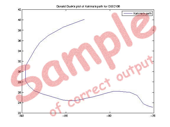
We can fix this by replacing our plot command with the following:

plot(-longitude,latitude);

Note how this corrects the shape of the plot. The correct plot should look more like this:

Step 3b: Making an script M-file, lab04a.m, that puts a plot on the web.

Now we are ready to make an M-File to do all this. You already have a file called lab04a.m in your account—this is mostly complete. This file adds several new commands to the ones we've learned already—here's an explanation of those:

• the close all command closes all currently open figure windows.
  • This is essential if we want to be able to run the script M-file more than once within the same MATLAB session.
• the legend command puts a legend on the graph.
  • Note that in the legend command, we put the message we want to appear in single quotes. If we need a single quote inside our message, we have to put two single quotes—not a double quote ("), but two single quotes ('')—so that MATLAB knows that the message isn't over yet.
• Example: legend('Katrina''s path');
• the title command puts a title at the top of the graph.
  • Example: title('Donald Duck''s map of Hurricane Katrina''s path');
  • We have the same issues here with single quotes.
• the form of the print command shown below sends the current MATLAB figure to a jpeg file.

Use either the MATLAB editor or emacs to edit the M-file lab04a.m, and make changes as follows:

• change Donald Duck to your name in both places where it appears
• change the section number 019 to your section number
• change the date 09/13/2007 to the actual date you finish the lab
• fill in the blank for the assignment statement that sets the variable latitude
  • If you skipped step 3a because you are doing this on a PC or Mac, you may need to skim through the instructions for step 3a for a hint about how to fill in this blank.
  • Another hint: consult the file katrina.txt for an explanation of which column is which. Don't just guess. If you do, you'll probably guess wrong.
  • after you do, delete the _______ characters that made the blank.
  • also delete the comment that says % FILL IN THE BLANK, THEN REMOVE THIS COMMENT

Producing the graph...

After you've typed in this and saved it, run it once to produce the graph. Remember that we run a script M-file by typing its name without the .m part (i.e. just type lab04a).

This week, you don't have to make a diary—instead, your plot on the web will be the evidence that your M-file works.

Halftime

If you've gotten this far, you are about half way done with this week's lab: you have two of the files you are going to submit.

In all, you are going to submit four files to WebCT: two M-files, and two jpeg files. Here is an overview:

Step 4: Make an M-file to plot wind speed vs. pressure

For the last step, I'm giving you only an overview of what to do. The detailed steps are up to you to figure out.

Fortunately, they are very similar to what you already did in Step 3, so you should be able to figure it out without too much trouble.

What to do:

1. From the instructions and guidance given in Step 3, determine what steps you should take to produce a graph of wind speed vs. pressure. Choose appropriate variable names and labels for a legend and title.
2. Make an M-file called lab04b.m that produces this graph, following the pattern given for lab04b.m.
3. Then run this M-file, and produce the graph, and save it as lab04b.jpg
4. Put it on the web as http://copland.udel.edu/~youruserid/cisc105/lab04/lab04b.jpg

When you've produce those two files, you are ready to submit.

Step 5: Submit the four files on WebCT.

You should upload and submit your two M-files, and your two JPEG files on WebCT—then, you are done!

Grading

1. lab04a.m (15 pts)
2. lab04a.jpg (15 pts)
3. lab04b.m (30 pts)
4. lab04b.jpg (30 pts)
5. Generally submitting everything according to instructions: 10 pts.

End of lab04 for CISC105, Fall 2007 (100 pts)
Due Date: 10/03/2007